
1 Introduction
Internet of Things (IoT) architectures are complex, involving many layers, including an application layer, a platform layer, a gateway layer, and an end-device layer [1]. Because of dynamic field conditions each layer must be able to communicate in various kinds of scenarios, including communication among end devices, communication between end devices and gateways, or communication between end devices and applications [2]. Each of these scenarios needs to be preceded by device pairing [3].
Initially, device pairing was done manually but now context-based zero-interaction methods [4] are used, one of which is dynamic device pairing. Dynamic device pairing is a term that describes that the pairing of two entities in an IoT architecture is carried out automatically [5,6]. This can be done by analyzing the received signal strength indicator (RSSI) values of the IoT entities to be paired. The RSSI describes the quality of the link between two wirelessly connected devices [7]. It can be used to make device pairing decisions: if the RSSI is getting stronger, which means the device is approaching, then pair; if the RSSI is getting weaker, which means means the device is distancing, then do not pair.
Reading the RSSI for device pairing can be problematic. If the device configuration is done at a high level, RSSI sampling cannot be performed at a high rate. As a result, it becomes more difficult to see whether the device is approaching or distancing. To increase the accuracy of dynamic device pairing of IoT end devices, this study proposes to use a hidden Markov model (HMM). An HMM is a Markov chain with hidden states and observed states [8]. This model can be applied by setting the RSSI as the observable state and the approaching or distancing state as the hidden state.
To prove the effectiveness of HMM implementation, this study investigated an IoT environment consisting of one smartphone, one access point, and one IoT end device. Four metrics were used to compare the performance of dynamic device pairing with HMM and without HMM: precision, recall, F1-score, and accuracy [9].
2 Literature Review
IoT device pairing has shifted from manual to context-based zero-interaction techniques. There are several reasons for this, two of which are security and efficiency. In terms of security, in 2016 a study was done on device pairing for crowdsourcing [10]. This study proposed a secure pairing method called Trustworthy Device Pairing (TDP). In 2017 a study was done on IoT device pairing with a proximity method to avoid attacks such as eavesdropping [11]. This was done by measuring the received signal strength indicator (RSSI) or signal strength when distancing, approaching, and turning.
Device pairing can be categorized as sensor-based and non-sensor-based. An example of sensor-based device pairing is the use of the inertial measurement unit (IMU) sensor on a smartphone combined with its camera [12]. Together, the two devices will detect motion; if the movements match, pairing will occur. In [12] images were used to detect movement, while [4] used sound. The assumption in the latter study was that two adjacent devices will have similar sound recording patterns when the sound source is the same (See Table 1).
Because sensors cannot always be used in context-based pairing, one study used time for pairing [13]. The idea behind this was that if two devices are close together, they have more similar timing compared to devices that are far apart. In enterpriselevel IoT, context-based pairing as discussed above takes a lot of time. The concept of context-awareness uses the shared history of two devices to decide whether they can pair or not [5].
| Device Pairing | Motivation | Context Aware | Method |
|---|---|---|---|
| Trustworthy Device Pairing | Security | No | Crowdsourcing |
| Anti-eavesdropping | Security | Yes | RSSI proximity |
| IMU-camera combination | Efficiency | Yes | Sensor-based |
| Sound context | Efficiency | Yes | Sensor-based |
| Similar timing | Efficiency | Yes | Time-based |
| Proposed method | Efficiency | Yes | RSSI proximity with |
| (this research) | HMM |
Table 1 Comparison of related works on device pairing.
3 Methodology
3.1 System Architecture
To test the performance of the proposed method, a testing environment was created comprising a smartphone, a Wi-Fi access point (AP), and an IoT end device. Figure 1 shows the topology of the IoT system.
Figure 1 The pairing architecture involving an IoT end device, a smartphone, and an AP.
Here, a smartphone with an Android operating system was used. Android Studio was used to develop the Android application. Figure 2 shows a sequence that describes the flow of the pairing system and the monitoring data transactions in general. The sequence diagram in Figure 2 starts with pairing. Pairing is initiated by the smartphone. If the pairing is considered valid, the IoT end device will reply with an ACK. If the pairing is successful, the smartphone can start pairing the end device with the AP.
Successful pairings are marked with ACK. If the end-device pairing with the AP is successful, the end device can begin sending monitoring data to the IoT platform via the AP. The data that are sent are temperature and humidity monitoring data. The monitoring data are collected on the IoT platform. If a user application on the smartphone wants to access these data, the user application can subscribe and the monitoring data will flow to the user application. The novelty of this research is the method for pairing the smartphone to the IoT end device and the IoT end device to the AP. Pairing is done by applying dynamic device pairing using HMM to increase the accuracy of the pairing.
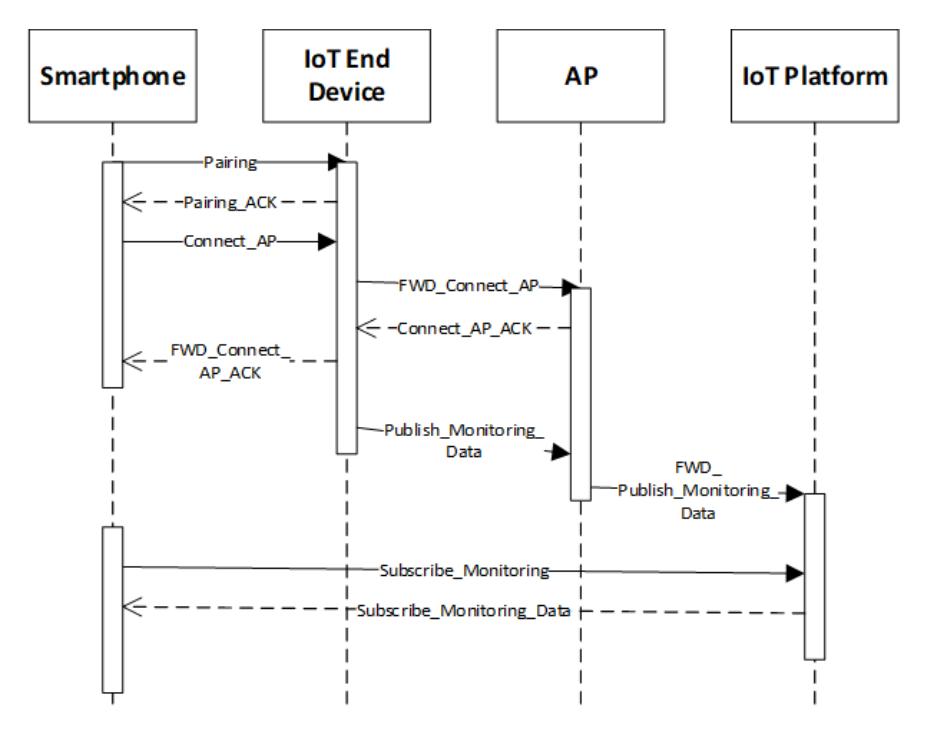
Figure 2 IoT end-device pairing sequence diagram.
3.2 Dynamic Device Pairing
Figure 3 describes the dynamic device pairing process [5]. The first thing to check is the history of the applications that want to pair. If the application has paired them previously, the application may do dynamic device pairing; if the application has never paired them before, the application must pair conventionally, like the process depicted in Figure 2. Dynamic device pairing is done by looking at the RSSI pattern of the application. If the pattern confirms that the application is approaching, the application is allowed to pair and the pairing will be executed automatically. If the RSSI is getting weaker or if it is detected as being silent, conventional pairing is executed. Here variations can be made, for example, if the RSSI is getting weaker over time, the pairing request can be rejected.
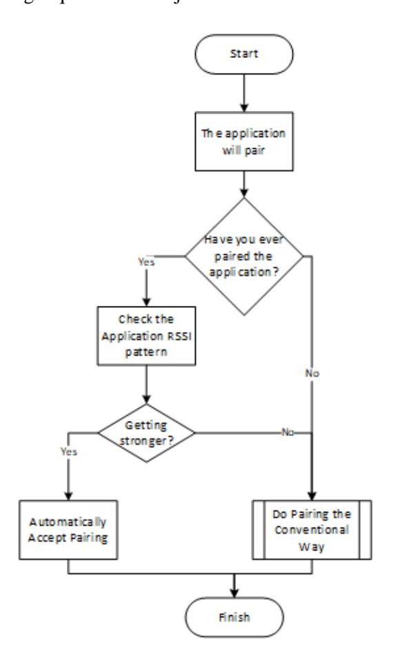
Figure 3 Flow chart of the dynamic device pairing algorithm.
3.3 Hidden Markov Model
HMM is an extension of the Markov chain. Both are used to calculate the probability of a sequence of events. The main difference between a Markov chain and HMM is that a Markov chain is used for fully observable cases, while HMM is used for cases involving hidden sequences [10]. Hidden Markov models can be used for pattern recognition applications, such as speech [14], writing [15], and body gestures recognition [16]. HMM can be used to solve problems that include
learning. HMM can also improve the accuracy of RFID reading sequences for a supply chain [17], which is an application similar to this research.
After the HMM has been successfully trained and modeled, the Viterbi algorithm is used to identify its hidden state [9]:
\[\delta(i) = \max_{q_1, q_2, \dots q_{t-1}} P[q_1, q_2, \dots, q_{t-1}, q_{t=i}, o_1, o_2, \dots o_t | \lambda]\] (1)
where δt(i) is the best series, q(i) is the hidden series, and o(i) is the observable series. The calculation follows several steps, namely initialization, recursion, termination, and path status. The following is the equation for initialization [9]:
\[\delta_1(i) = \Pi_i b_i(o_1), \ 1 \le i \ge N\] \[A_r(1) = 0. \tag{2}\] where Πi is equal to the initial probability, bi(o1) is equal to the first element of the observed state probability output, 1 ≤ i ≥ N is the range where i is the state and N is the number of states, Aґ (1) is set to 0 and is equal to the first transition probability value.
In the recursive stage, a repetition process is carried out on the process itself using the following equation:
\[\delta t(i) = \max \left[ \delta t - 1(i) a_{ij} \right] b_j(o_t) \text{ for } 1 \le i \le N, \tag{3}\] where t-1(i) is the last time in the time series with state I; aij is the transition probability from i to j, and bj is the state that is equal to the density probability.
In the termination stage the following equation is executed:
\[P^* = \max \left[ \delta T(i) \right] \text{ for } 1 \le i \le N. \tag{4}\] where P* is the decision stage carried out, which is determined from the maximum observation sequence value.
The status path state determines the final output.
Four metrics were used to measure the performance of the HMM method in increasing detection accuracy in dynamic device pairing, namely recall, accuracy, precision, and F-measure. The following are the equations for each metric [9]:
\[Recall = \frac{TP}{TP + FN} \tag{5}\]
\[Accuracy = \frac{TP + TN}{TP + TN + FP + FN} \tag{6}\]
\[Precision = \frac{TP}{TP + FP} \tag{7}\]
\[F - Measure = 2 x \frac{Precision x Recall}{Precision + Recall}\] (8)
where TP is true positive, TN is true negative, FP is false positive, and FN is false negative.
4 Result
To test the success of HMM in increasing detection accuracy in dynamic device pairing, a test system was built, consisting of an AP, a smartphone, an IoT platform, and an IoT end device. The IoT end device consisted of a NodeMCU microcontroller that could send temperature and humidity data to the IoT platform [18]. For the smartphone an application was created using Android Studio. The system that implements the sequence in Figure 2 was successfully created. Furthermore, the algorithm for dynamic device pairing shown in Figure 3 was also successfully created. Next, HMM was implemented to improve detection accuracy in dynamic device pairing.
To create the HMM model, a data set was created. A total number of 100 data were collected by making 100 smartphone movements on the IoT device. The data set was divided into 50 distancing movement data and 50 approaching movement data. For each move, the RSSI value before movement and after movement wasrecorded. Table 2 shows the data set specifications. The total amount of data was considered representative for testing. Additionally, it must be noted that the data set gathered did not contain unreliable data, omitted data, duplicated data, bad labels, or bad values.
Table 2 Dataset specification.
| Class Name | Amount | Feature 1 Name | Feature 2 Name | |
|---|---|---|---|---|
| Class 1 | Approaching | 50 | Initial RSSI | Final RSSI |
| Class 2 | Distancing | 50 | ||
| Total number of data | 100 |
The data set then went through a training process to form the HMM model. The HMM model produced by training can be seen in Figure 4. Figure 4 describes the probability of displacement between movements that occurred in the system based on the collected test data.
For testing, two types of motion were used. These movements were labeled as approaching or distancing. The approaching and distancing movements were carried out over a distance of 30 cm with a constant speed of motion, namely 0.1 meter per second in 3 seconds.
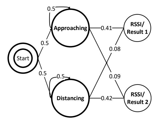
Figure 4 The HMM model.
Figure 4 is the HMM state used with the initial probability value, the probability between movements, and the probability of movement towards RSSI. Two movements were used so there were two RSSI results. The initial probability was obtained from the value of each movement when it started. The probability between movements was obtained from the value of the displacement caused by the smartphone's movement.
Next, a comparison of the two methods was made. The first method was used to identify movements based on the algorithm in the flowchart in Figure 2 and the second method was used to identify movements with the HMM model that had been created. Both tests used the created data set. The data were classified into TP, TN, FP, or FN. Table 2 provides an explanation of each category.
Category Explanation TP Actually approaching and predicted as approaching TN Actually distancing and predicted as distancing FP Actually distancing but predicted as approaching FN Actually approaching but predicted as distancing
Table 3 Dataset specification.
The results of the categorization of the two methods are presented in separate confusion matrices [19]. The confusion matrix without HMM can be seen in Table 3 and the confusion matrix with HMM can be seen in Table 4. In Table 4, pairing without HMM produced 47 TPs, 28 TNs, 22 FPs, and 3 FNs. The total number of predicted positives was 69 and the total number of predicted negatives was 31.
Table 4 Confusion matrix without HMM.
| Predicted | |||
|---|---|---|---|
| P | N | ||
| Actual | P | 47 | 3 |
| N | 22 | 28 | |
In Table 5, pairing with HMM produced 47 TPs, 41 TNs, 9 FPs, and 3 FNs. The total number of predicted positives was 66 and the total number of predicted negatives was 44.
Table 5 Confusion matrix with HMM.
| Predicted | |||
|---|---|---|---|
| P | N | ||
| Actual | P | 47 | 3 |
| N | 9 | 41 | |
From the results in the confusion matrices in Tables 4 and 5, the performance of each method was calculated using the metrics mentioned in Equations (5) to (8). The results are compared in the bar chart in Figure 5.
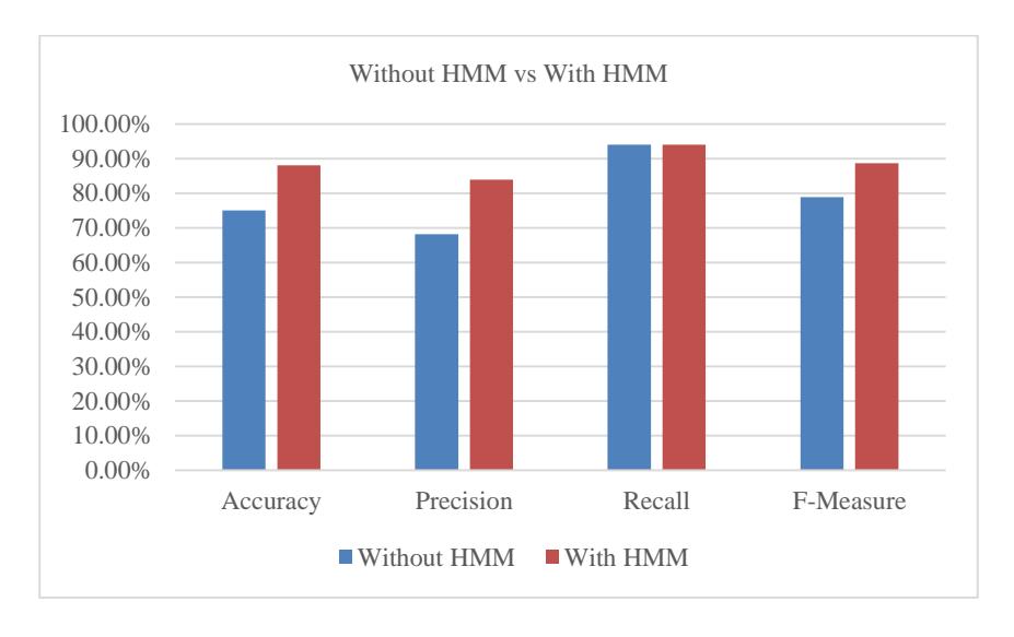
Figure 5 Performance comparison between dynamic device pairing without HMM and with HMM.
The dynamic device pairing with HMM performed better in terms of accuracy, precision, recall, and F-measure. Accuracy for dynamic device pairing without HMM was 75%, while with HMM it was 88%. Precision for dynamic device pairing without HMM was 68.12%, while with HMM it was 83.93%. Recall for dynamic
device pairing without HMM was 94%, while with HMM it was 94%. F-measure for dynamic device pairing without HMM was 78.9%, while with HMM it was 88.68%.
According to our analysis, HMM did not improve recall performance but did significantly improve precision. Increasing precision is equivalent to decreasing the FP value. When the FP rate, also called the false alarm rate, is high it indicates that the predictor is too sensitive in detecting positive values. Thus, HMM was able to reduce this sensitivity.
The increase in accuracy, precision and F-measure when using HMM is because HMM is successful in predicting the probability of moving from one state to another until it reaches the goal state. The displacement probabilities can be determined by looking at the observation variables, namely approaching and distancing. For the hidden variable, the RSSI results also have an effect on the calculated displacement between states. For example, HMM can be used if someone wants to know the value of the probability of displacement from the approaching observation variable toward hidden variable RSSI 1. Thus, HMM can improve the prediction accuracy of the system proposed in the study. This makes HMM usable for a broader range of IoT systems. With HMM, the accuracy of dynamic device pairing can be improved. The motivation for implementing dynamic device pairing using HMM is to improve the performance of enterprise-scale IoT, for example in smart classrooms, smart lighting, smart buildings, and other applications. Considering the improved dynamic device pairing performance of the HMM method, in a future research this system will be tested on an enterprise-scale IoT system.
5 Conclusion
A hidden Markov model was successfully applied to the dynamic device pairing of an IoT end device based on changes in RSSI. The tests showed that dynamic device pairing with HMM could improve performance compared to dynamic device pairing without HMM. The accuracy of dynamic device pairing without HMM was 68.12%, while it was 83.93% with HMM. In a future work, this method will be tested on an enterprise-level IoT system.
Acknowledgement
The authors would like to thank Telkom University for funding this research.