
1 Introduction
In data analysis tasks, the use of a large amount of data in high-dimensional datasets directly affects performance because irrelevant and redundant features also contribute to the analysis. To overcome this problem, these irrelevant and redundant features should be eliminated, leading to more effective dimensions. This data preprocessing step is called feature selection. Generally, the goal of feature selection is to determine the best subset of features for conducting statistical analysis or building a machine learning model. Feature selection assists in selecting the minimum features from the whole dataset. To ensure an optimal feature subset, a feature selection method has to evaluate a total of 2n – 1 subsets, where n is the total number of features in the dataset. Even though this exhaustive search for the optimal feature subset results in an optimal solution, it is not very practical, especially with moderately large values of n.
This type of problem is said to be an NP-hard problem and many search strategies for suboptimal solutions have been proposed in the literature. Feature selection algorithms can be classified in many different ways. According to [1- 3], the most common ones can be categorized into three types, that is the filter approach, the wrapper approach, and the embedded approach.
The filter approach uses an independent criterion function to select features without depending on the type of classifier used, which leads to a simple method, while the interactions with classifier and feature dependencies are ignored. The filter method ranks each individual feature according to measurements such as information, distance or similarity. It only considers the association between the feature and the class label. The nature of this method results in a drawback, namely that all features are considered separately.
The wrapper approach uses the result of the classifier to determine the goodness of the given feature, therefore the selected features are dependent on the classification algorithm. This method removes the disadvantage of the filter approach by considering feature dependencies, but it is more time-consuming than the filter approach. The quality of the feature subset is directly related to the performance of the classifier.
The embedded approach searches for the optimal feature subset during the model training that is built into the construction of the classifier. It returns both the learned model and the selected features simultaneously. The benefit of this method is that it takes less computational time than the wrapper approach. This method is also called the hybrid model. It incorporates a learning algorithm and is optimized for higher accuracy. The embedded approach utilizes a filter-based technique to select highly representative features and then applies a wrapperbased technique to add candidate features. The candidate subsets are evaluated for selecting the best ones. This does not only reduce the dimensionality of the dataset but also decreases the computational time and improves the performance. Somol, et al. in [4] have proposed the flexible hybrid Sequential Forward Floating Selection (hSFFS) method by employing an evaluation function to filter some features and using a wrapper criterion to identify the optimal feature subset. The main benefit of this method is the ability to trade off the resulting quality with the computational cost in order to enable wrapperbased selection in highly dimensional datasets. The experimental results showed promising classification accuracy.
In this research, we explored an effective way to improve the classification accuracy of a machine learning model regarding sequential feature selection. Our method employs an adaptive multi-level backward search to maximize the resultant feature subset. The methodology of the proposed feature selection
method is presented along with a comparison against other sequential feature selection techniques on twelve standard UCI datasets. We conclude our paper by giving some directions for further research in the last section.
2 Related Work
2.1 Feature Selection
Feature selection is a necessary step in the data mining process because the high dimensionality and vast amount of data is a challenge in learning tasks. Many irrelevant features do not add much value during the learning process, hence learning models tend to become highly complicated and decrease learning accuracy. Feature selection is one effective way of identifying relevant features for dimensionality reduction. However, the benefit of feature selection comes with an extra effort when trying to get an optimal subset that represents the original dataset.
Jovic, et al. [5] categorize feature selection methods into three common search strategies. Exponential algorithms evaluate subsets that grow exponentially with the feature space size, for example exhaustive search and branch-and-bound. Sequential algorithms such as SFFS include or exclude features from the active subset sequentially. Random algorithms incorporate randomness into the search process to optimize the solution. An example of random algorithms are evolutionary computation algorithms using genetic or ant colony optimization. A recent study from Homsapaya & Sornil in [6] introduced a floating search technique employing a genetic algorithm (GA) to improve the quality of the selected feature subset. The results showed that GA improved the performance for the majority of sample datasets. Kadhum, et al. in [7] have proposed a new model for evolutionary wrapper feature selection by applying GA to explore the space of feature combinations from a set of features that already has its priorities assigned. Extreme Learning Machines (ELM) and Support Vector Machine (SVM) were used as the classifiers based on the Chronic Kidney Disease dataset (CKD) from the UCI repository. The application of the proposed model affected the classification performance by improving the accuracy rate while also reducing the computing time.
Seeing that there is no optimization technique that is suitable for all feature selection problems, Ref. [8] presents a systematic literature review on the subject of multi-objective feature selection based on numerous multi-objective techniques and algorithms in order to help researchers find the best approach for their work. The study also showed that the majority of feature selection methods apply the wrapper method combined with supervised learning classification. Wan, et al. [9] proposed a novel discrete sine cosine algorithm (SCA) for multiobjective feature selection to trade off between information preservation and redundancy reduction. Their experiments on ten UCI datasets showed the superior capability of discrete sine cosine algorithm-based multi-objective feature selection (MOSCA_FS), which was confirmed with all the tested datasets. The important study by Al-Tashi, et al. in [10] applied a binary version of the Multi-objective Grey Wolf optimizer (MOGWO) based on a sigmoid transfer function called BMOGW-S. Its classification performance using a wrapper artificial neural network (ANN) was compared with MOGWO with a tanh transfer function, the Non-dominated Sorting Genetic Algorithm (NSGA-II), and Multi-Objective Particle Swarm Optimization (MOPSO) on fifteen standard UCI datasets. The results showed that BMOGW-S outperformed the other techniques in both feature reduction and classification accuracy.
A similar study on sequential feature selection in [11] introduced an adaptive Multi-level Forward Inclusion (MLFI) method, which focuses on the searching space in the forward direction by looking ahead for some specific level of generalization limits. Our study attempted to discover a better subset in the backward direction. A k-nearest neighbor classifier (k = 5) was applied in the performance validation using eight UCI datasets. The MLFI algorithm showed better performance than the other sequential forward searching techniques for the majority of the results.
Other recent works in the feature selection domain focused on the application of feature selection techniques to other areas of work, such as face recognition, text classification and medical science [12-14]. The improvement of sequential feature selection tends to focus on non-deterministic algorithms like particle swarm optimization, genetic algorithms or deep neural networks in [15] and [16], while our study concerned a deterministic algorithm.
Our research focused on a wrapper approach based on sequential feature selection algorithms. The proposed method uses the result of a data mining algorithm to determine the goodness of a given subset. During the search process, the space of possible feature subsets is defined to generate and evaluate features until we get the optimal subset. For the sequential floating search methods, the number of features dynamically increases and decreases until the desired target is reached.
The variables allow floating forward or backward so they can be flexibly changed without presetting any parameters. Because of this, a nesting effect may occur since the best k-subset does not necessarily contain the best (k–1) subset. Therefore, we made an improvement to the floating search algorithm to remove some of its drawbacks and tried to find a solution that is as close to the optimal solution as possible.
2.2 Sequential Forward Search
The sequential forward search (SFS) [17] process in a forward search manner starts with an empty set and adds one feature to the selected subset during each iteration until a new feature subset is discovered that maximizes the criterion function value. SFS is essential for constructing other more complex algorithms. Large datasets normally contain many features, whereas only some of them are significant for model training. The idea is to select the feature subset that gives the highest learning accuracy. Assume we have a set Y = {y1, y2,…, yD}, where D is the number of input dimensions. We want to find a subset Xk = {xj | j = 1, 2,…, k; xj Y}, where k = (0, 1, 2,…, D), and d is the required subset size. Initialize X0 = {} and k = 0, and x + is an included feature where x Y – Xk. The algorithm can be described as follows:
Step 1: Inclusion step.
          x
           + = arg max J(xk = x), where x  Y – Xk
          Xk+1 = Xk + x
                       +
          k = k + 1
          (Add a selected feature x
                                     +
                                       to subset Xk, where x
                                                              +
                                                                is a feature that
maximizes the criterion function (J).) Step 2: Continue step 1 until d features are selected.
2.3 Sequential Forward Floating Selection
One of the most significant innovations in this area is the Sequential Forward Floating Selection (SFFS) proposed by Pudil, et al. in [18]. This technique combines the concept of SFS with sequential backward search (SBS). SBS gives it more effectiveness than SFS by introducing a backtracking step. The SBS method starts with a full feature subset and eliminates one feature in each iteration until a predetermined criterion is satisfied.
The backtracking step is a conditional step, where an improvement can be made during the search process. SFFS is said to be a state-of-the-art method that is widely used in several applications. Researchers in sequential feature selection normally extend their method using SFFS as the standard method to compare their results. To explain the SFFS algorithm below, let x – be an excluded feature where x Xk.
Step 1: Inclusion step (apply the SFS algorithm).
Step 2: Conditional exclusion step (this step is similar to the SBS algorithm).
x
 – = arg max J(xk = x), where x  Xk
If J(xk – x
          –
           ) > J(xk–1):
       Xk–1 = Xk – x
                     –
       k = k – 1
(Remove a feature if the resulting subset improves the performance. If k 2 or there is no improvement, go to step 1, else repeat step 2.)
Step 3: Continue steps 1 and 2 until d features are selected.
After the introduction of SFFS, several improved versions have been proposed to obtain better performance. An adaptive version of the floating search method was presented by Somol, et al. in [19]. The idea behind Adaptive SFFS (ASFFS) is selecting features to add or remove more than one feature in each sequential step in order to search for a better subset. The number of search features in each step can be varied depending on the remaining features in the dataset. The result is a more thorough search with a better chance of finding an optimal solution by setting a higher generalization level. There are two free parameters, rmax and b, in ASFFS that specify the generalization limit and range of the adaptive search. The parameter r specifies the number of features to be added in the forward phase or inclusion phase and is calculated adaptively. The backward phase or exclusion phase removes o features if it increases the performance. ASFFS is identical to SFFS if we assign rmax = 1. The suggestions for the two values are 4 and 3, respectively. The nearer the current subset size to d, the higher the generalization limit. The reason behind this characteristic is to save time by limiting the generalization level while the current subset is still far from the desired one. The generalization level (r) increases when the number of features (k) in the current subset gets close to d until it reaches rmax. ASFFS has shown better results than SFFS due to a more thorough search.
Calculation of the r value is done at the beginning of every forward and backward phase using the following conditions:
1. If |k – d| < b, let r = rmax
- 2. Else if |k d| < b + rmax, let r = rmax + b |k d|
- 3. Else let r = 1
While the number of features is far from the required subset size, r is assigned a value of 1, which is exactly the same as SFFS's procedure. When k gets closer to d, the value for r increases but no more than rmax. Even though ASFFS has shown slightly better results than SFFS, it takes more computational time due to the complexity of the algorithm. The adaptive step leads to additional work to the SFFS structure both in the forward and the backward direction. Elements of the current feature subset can be increased or decreased along the searching process, which is another reason for the longer time required. The generalization level can be helpful during the search only when k in the current subset is getting close to the target size, thus the detailed search concept works only when k almost reaches the end of the process.
2.4 Improved Forward Floating Selection
Improved Forward Floating Selection (IFFS) was introduced by Nakariyakul & Casasent in [20], which successfully removed the weakness of SFFS by adding an additional step to improve the criterion function value. Based on the fact that it is not necessary that the best k-subset contains all features from the best (k–1) subset, IFFS was introduced. This improved step is called 'replacing the weak features', that is to check whether removing any feature in the currently selected feature subset and adding a new one at each sequential step can improve the current feature subset.
IFFS can impressively prevent the nesting effect of SFFS and the algorithm is simpler than ASFFS with an exceptionally short computing time. IFFS yields better performance than both SFFS and ASFFS with a little more process time than SFFS. The IFFS algorithm is described below, applying the same variables as SFFS:
Step 1: Inclusion step (apply the SFS algorithm).
Step 2: Conditional exclusion step (apply the SBS algorithm).
Step 3: Check if replacing a weak feature helps.
For xi in Xk :
       Xk–1 = Xk – xi
       For xj in Y  Xk–1 :
              xj = arg max J(xj)
              If J(Xk–1+ xj) > J(Xk):
                     Xk = Xk–1+ xj
(Generate k new subsets of k features by removing one feature and adding one feature using SFS. Calculate the J-values of k-subsets. If the subset with the largest J-value gives an improvement, then replace the new subset with the current subset and go to step 2. Otherwise, go to step 1.)
Step 4: Continue steps 1, 2 and 3 until d features are selected.
3 Proposed Method
Feature selection using the wrapper approach is more of interest due to the high classification accuracy when compared with other approaches. Several methods apply the wrapper approach to sequential feature selection. The most popular sequential search algorithm is SFFS, which represents the standard method. Other techniques are usually developed from SFFS in order to improve classification accuracy with a reasonable time complexity and also to overcome the effect of the nesting problem. The development of ASFFS and IFFS has been shown to be superior to the standard SFFS.
In our study, we present One-level Forward Multi-level Backward Selection (OFMB), which is a sequential forward selection method that explores possible subsets several levels deeper in order to maximize the classification accuracy of the learning dataset. The idea is to explore backward after feature inclusion since newly included features may affect smaller subsets. This backward search can examine many levels by excluding more than one feature in each iteration. This method considers a wider range of features when searching backwards deeper. OFMB is similar to the backtracking step of SFFS but it can explore feature subsets to much greater depth. Subsequently, a new, smaller subset with a higher criterion function can be discovered, whereas the standard SFFS or even IFFS are not capable of finding such subsets.
This is a description of the OFMB algorithm:
- Step 1: Apply SFS to select one feature from the remaining feature set. Add this feature to the selected feature subset. Continue step 2 with the feature subset Xk where k = k + 1.
- Step 2: From the selected feature subset size k, remove 1 feature iteratively. We have Xk–1 and use SFS to select a new feature from the remaining feature set (Y Xk–1) for adding to each feature subset. Then calculate whether there is an improvement. If there is an improvement, replace that previous feature subset with the newly selected feature subset and repeat step 2. Otherwise, continue step 3 with feature subset Xk.
- Step 3: From the selected feature subset (Xk), remove s features iteratively from 1 to r. Then, search for the best (k–s)-subset. If there is a better subset Xk–s, then replace it with the previous Xk–s. Repeat steps 3 until s > r, then continue step 4.
- Step 4: Compute the r value, then continue step 5.
- Step 5: Continue steps 1, 2, 3 and 4 until d features are selected.
From Figure 1, starting with an empty set, first we add features using SFS until we get more than two features and then the process can continue to include features according to which feature can give a higher J value for a subset of size k. This process allows the number of features to be either increased or remain the same without a backtracking step. The insertion of 'replacing a weak feature' from IFFS during the forward phase makes it possible to improve the feature subset and remove the nesting effect problem. While using SFS to include one feature, we try to find a better feature subset by removing one feature in that subset for every element except the one that has just been added. If an improvement can be made, replace the new subset with the current one. If there is no improvement, we will add another feature in the next iteration. This is a feature improvement step that applies a technique from the IFFS algorithm.
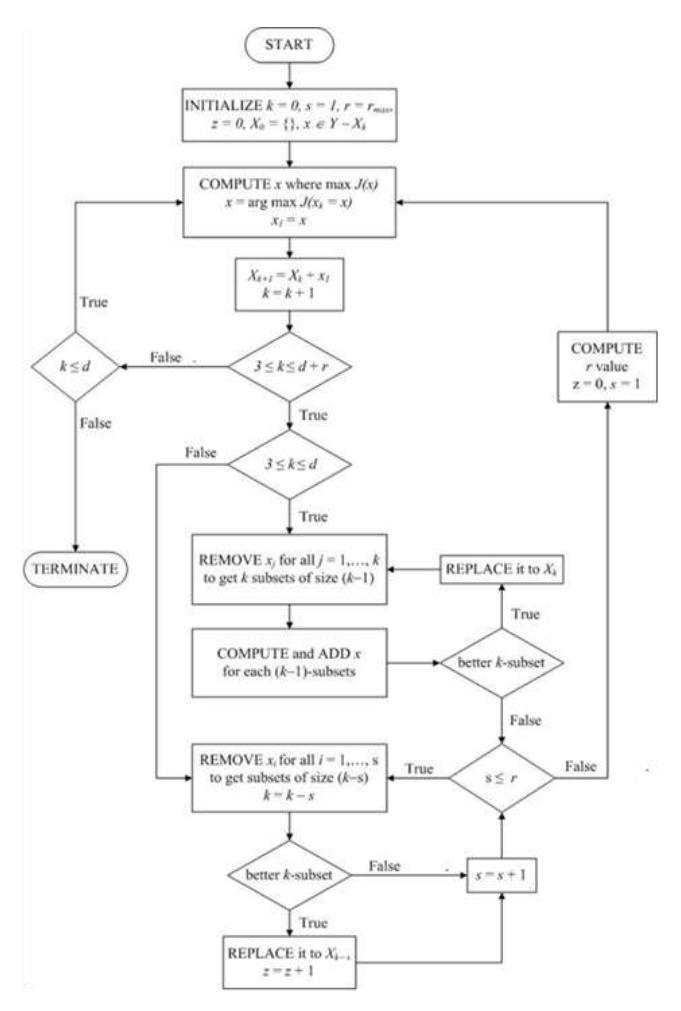
Figure 1 Flowchart of the OFMB algorithm.
The first phase of OFMB consists of constructing a set of feature subsets that have relatively high classification accuracy, similar to IFFS. The second phase consists of exploring the last selected subset deeper backwards, up to some specified point. After the inclusion and improvement steps, we remove one or more features from the currently selected subset to form many subsets of size (k–s), where s refers to the number of removed features ranging from 1 to r, and r is the generalization limit. The searching target is a subset with a higher J value for a particular subset size. We propose the conditions used to calculate the value of r in the next subsection. As a result of applying the OFMB technique, there is a better chance of finding a better feature subset of size (k–s). Pseudo code for the OFMB algorithm is provided below.
Algorithm: One-level Forward Multi-level Backward Selection (OFMB) Input: A set of features Y = {y1, y2,…, yD}, where D is the number of input dimension; J is a criterion function; d is the required subset size; r is the generalization level, which is limited by rmax. Output: A feature subset Xk = {xj | j = 1, 2,…, k; xj Y}, where k = (0, 1, 2,…, d). Initialize: Initialize X0 = {}; k = 0; s = 1; r = rmax; z = 0. (1) Feature Inclusion #Find the best feature and update Xk x + = arg max J(xk = x), where x Y – Xk Xk+1 = Xk + x + k = k + 1 max(Xk) = Xk+1 (2) Feature Improvement #Replace weak features by removing one and adding one Repeat For xj in Xk : #where j = 1, 2,…, k Xk–1 = Xk – xi For xi in Y Xk–1 : #where i = 1, 2,…, d (k–1) xi = arg max J(xi) If J(Xk–1+ xi) > J(Xk): Xk = Xk–1+ xi max(Xk) = Xk Until J(Xk–1+ xi) J(Xk) (3) Multi-level Backward Selection #Searching for better subsets by multiple backtracking step Repeat xs in Xk : #where s = 1,…, r and xs are the features from 1 to r Xk–s = Xk – xs If J(Xk–s) > J(max(Xk–s)): max(Xk–s) = Xk–s z = z + 1 s = s + 1 Until s > r (4) Compute r-value If z < rmax : r = rmax – z Else : r = 1 z = 0 s = 1 (5) Termination Condition #Terminate when k > d If k d
Go to step 1 Xk = max(Xk) #for all k
Return the best individual subset Xk
We can see that the subset increases in size along with an improvement across the process until it reaches the required value of d. This method also solves the nesting problem that occurs in SFFS and produces a result equal to or greater than IFFS without backtracking step. Our proposed method solely consists of three main parts, that is Feature Inclusion, Feature Improvement, and Multilevel Backward Selection. The first two parts provide preliminary results for the multi-level backward tracking, which is the technique that most noticeably improves the performance in terms of classification accuracy. The criterion functions (J) can be calculated using the classifiers described in Section 4.1.
3.1 Computation of r Value
The generalization limit (r) needs to be carefully specified since a larger value of r results in a more thorough search, which increases the time complexity. We introduce a user-defined parametric limit, rmax, to restrict the maximum generalization level. This number can be any integer depending on how deep we need to search, but normally it is only a small integer. In our experiments, we assigned the value of rmax to be 5 for all tested datasets. Level s is similar to level o in the ASFFS method, where s is determined dynamically according to the r calculation technique we propose.
The generalization limit can change adaptively depending on the number of times we have found better k-subsets. If we have found a small number of better subsets in the previous iteration, then we should try a deeper search in the next iteration, which will increase the value of r. On the other hand, if the previous iteration found many better subsets, the next iteration should not need to go too deep, decreasing the value of r. Conversely, the search should go deeper when it cannot find a better subset. The application of this calculation technique leads to better performance than the previous works. We have selected the first 20 features from the whole dataset for the experiments. OFMB considers a wider range of features, which leads to a thorough search. As a result, it has a better chance of improving the current feature subset.
Assume rmax = 5, thus 1 r 5. Let z be the number of times the algorithm has found a better subset for that particular iteration. Suppose that z is related to r by rmax – z. Adaptive determination of r is defined as follows:
1. If z < rmax, let r = rmax – z
2. Else, let r = 1
From the condition above we can build the graph in Figure 2, which shows the value of r for the first 20 features; if we have z = {0, 0, 2, 0, 3, 0, 2, 0, 0, 0, 3, 0, 2, 1, 0, 0, 3, 0, 4, 0}. The example of the z values come from the Ionosphere dataset. The value for r decreases while z increases.
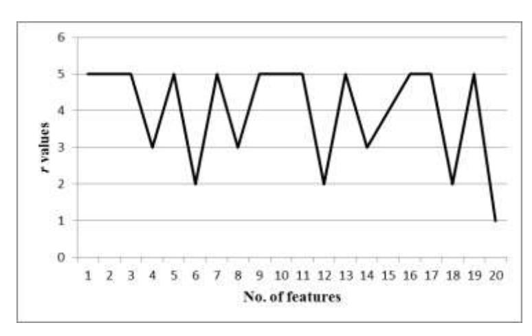
Figure 2 Graph of r values.
3.2 An Example Using the Wine Dataset
To demonstrate the OFMB algorithm, we selected the Wine dataset from the UCI repository based on the KNN classifier. First, assume we have a dataset Y = {0, 1, 2, 3, 4, 5, 6, 7, 8, 9, 10, 11, 12} with 13 features; the required subset size (d) is 20 features, and we assign rmax = 5. Since the Wine dataset contains only 13 features, we need to process until d = 13, and we have z = {0, 0, 0, 0, 0, 2, 0, 1, 2, 0, 0, 0, 0}.
3.2.1 Feature Inclusion
At the beginning, assume we apply SFS for the first 3 features, thus for k = 1, 2 and 3 we have X1 = {6}, X2 = {6, 10} and X3 = {6, 10, 2} respectively. Now, the current subset of k = 3 is X3 = {6, 10, 2}. This subset is the best 3-subset that has been found so far.
3.2.2 Feature Improvement
Assume we continue the process up to k = 4. We have X4 = {6, 10, 2, 7} with 90.09% classification accuracy. Remove one feature except x4 = 7 and we have {6, 10, 7}, {6, 2, 7} and {10, 2, 7}. Then, select one feature from the remaining set that produces the best J value with those 3 subsets. Now we have new subsets of size 4 for consideration. After calculation we find that J({10, 6, 7, 9}) produces the highest J value with 92.84% accuracy. Therefore, replace {6, 10, 2, 7} with {10, 6, 7, 9} as the best subset of size 4 that has been found so far. Repeat the same process for X4 = {10, 6, 7, 9} and we cannot find any better subset, thus we continue to the next step with X4 = {10, 6, 7, 9}. The next step will be an optimization of this solution.
3.2.3 Multi-level Backward Selection
Assume we continue the process until we reach k = 9 and we have X9 = {0, 1, 2, 5, 6, 9, 10, 7, 8} with 92.25% accuracy. After the feature improvement step we have X9 = {0, 1, 2, 5, 6, 7, 8, 9, 11} with 92.82% accuracy that is the best 9 subset that has been found so far. For Multi-level Backward Selection, starting with s = 1, remove one feature to find a better 8-subset. Now we consider only subsets containing the feature x9 = {8}, which are {0, 1, 2, 5, 6, 7, 8, 11}, {0, 1, 2, 6, 7, 8, 9, 11}, {0, 1, 2, 5, 6, 7, 8, 9}, {1, 2, 5, 6, 7, 8, 9, 11}, {0, 1, 2, 5, 7, 8, 9, 11}, {0, 1, 2, 5, 6, 8, 9, 11}, {0, 2, 5, 6, 7, 8, 9, 11}, {0, 1, 5, 6, 7, 8, 9, 11}. We calculate the J values for all the combinations of 8-subset but cannot find a better 8-subset. The process continues to the next inner loop for s = 2. Remove two features from X9 = {0, 1, 2, 5, 6, 7, 8, 9, 11} and we have {0, 2, 5, 6, 8, 9, 11}, {2, 5, 6, 7, 8, 9, 11}, {0, 2, 5, 7, 8, 9, 11},…, {0, 5, 6, 7, 8, 9, 11} for 28 subsets of size 7 to be considered. The calculation has shown no better result, thus continue to the next inner loop for s = 3. Remove three features from X9 = {0, 1, 2, 5, 6, 7, 8, 9, 11} and we have {1, 2, 6, 7, 8, 11}, {0, 1, 2, 6, 8, 11}, {1, 2, 5, 6, 8, 11},…, {2, 5, 6, 7, 8, 11}. There are 56 subsets of size 6 to be considered. At this point, we can find a better 6-subset, which is {0, 6, 7, 8, 9, 11} with 93.36% accuracy. Replace X6 with {0, 6, 7, 8, 9, 11} as the best 6 subset that has been found so far. From Figure 3 shows that X6 now has the highest accuracy, which cannot be found by other sequential searching techniques.
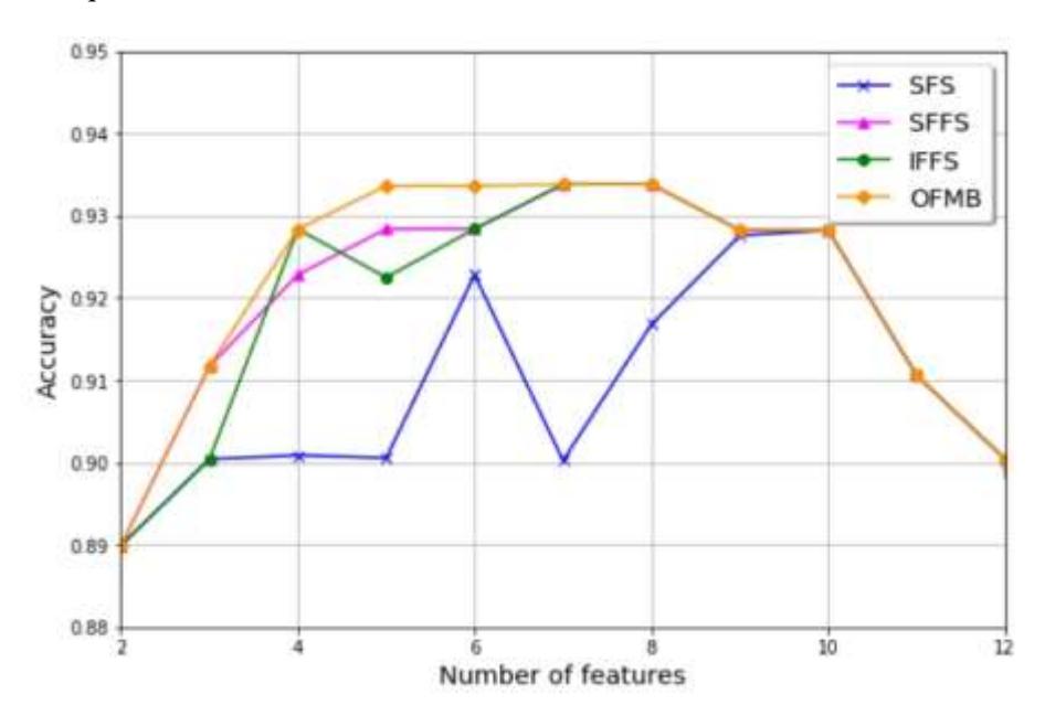
Figure 3 Accuracy graph for Wine dataset using KNN.
3.2.4 Compute the r Value
An adaptive determination of r is applied to find the value of r for the next iteration. There are two input variables: one is the maximum value of r (rmax), which is 5 for this particular example. The other one is z, which has recently been acquired from the multi-level backward selection step. If k = 6, the value of z would be 2. Apply an adaptive determination of r that matches with the first condition, which is 'If z < rmax, let r = rmax – z'. Thus we have r = 5 – 2 = 3. Now, r = 3 will be applied to the algorithm for k = 7. The value of r can vary from 1 to 5 depending on the value of z. Therefore, r changes adaptively in different iterations.
3.2.5 Termination Condition
The OFMB algorithm processes sequentially until the subset size (k) reaches the required subset size (d). The best of all feature subsets are copied into Xk and the program is terminated. This method applies the idea of adaptive search in order to explore the potential subset thoroughly, in other words, it provides a better chance of finding the optimal solution via a more detailed search by adjusting the generalization limit adaptively.
4 Experimental Evaluation
4.1 Experimental Setup
To compare our method with other algorithms we developed an experimental environment similar to previous works. The performance of feature selection methods is usually evaluated by a machine learning model. Due to the robustness and versatility of the k-nearest neighbor (KNN) classifier, it is used in various applications that can outperform other more powerful classifiers. Therefore, we decided to use KNN to compare our performance with different sequential floating feature selection algorithms.
The naïve Bayes (NB) classifier is the other classification model we selected. It is based on probability theory by applying Bayes' theorem. It has been used widely in machine learning research since the 1950s because of its effectiveness and ease of implementation without complicated iterative parameter estimation. The NB classifier often outperforms more sophisticated classification methods. We used KNN and NB to compare our method's performance on different algorithms based on 5-fold cross-validation. Data normalization is preferred as a preprocessing step. We selected Python as the programming language, using the Jupyter notebook editor for program development.
Table 1 shows the twelve standard datasets with various sizes from the UCI repository used in this research to evaluate our results. We randomly selected some instances for a large dataset and also eliminated some missing values when necessary. We applied the same randomly selected instances to all techniques to ensure that they received the same input.
| Name | Feature Type | No. of instances | No. of features | No. of classes |
|---|---|---|---|---|
| Wine | Integer, real | 178 | 13 | 3 |
| Thoracic Surgery | Integer, real | 470 | 17 | 2 |
| Online Shoppers | Integer, real | 12330 | 17 | 2 |
| Lymphography | Categorical | 148 | 18 | 2 |
| Image Segmentation | Real | 2310 | 19 | 7 |
| Crowdsourced | Real | 10546 | 29 | 6 |
| Breast Cancer | Real | 569 | 32 | 2 |
| Ionosphere | Integer, real | 351 | 34 | 2 |
| Soybean | Categorical | 307 | 35 | 15 |
| Spambase | Integer, real | 4601 | 57 | 2 |
| Sonar | Real | 208 | 60 | 2 |
| Urban Land Cover | Real | 675 | 147 | 9 |
Table 1 Datasets used in the experiments.
4.2 Results and Discussions
In this section, we discuss our results for the OFMB algorithm compared with popular suboptimal methods, that is SFS, SFFS and IFFS. This research aimed to increase the classification accuracy rather than reducing the time complexity. The size of the dataset does not affect the algorithm. The number of features calculated from each dataset would be either 20 or less depending on the size of the dataset. We studied the effectiveness of the proposed sequential feature selection algorithm based on two classification methods, that is KNN and NB, on twelve standard UCI datasets. Their performance was evaluated by classification accuracy and the minimum number of selected features that produced the maximum accuracy. The classification accuracy is the first priority for the best performance. If the accuracy results for the different algorithms were equal, then the smallest number of selected features was considered.
The results in Table 2 show that the classification accuracy was noticeably enhanced by the proposed algorithm compared to the previous works using KNN as performance validation method. OFMB had the best performance in the majority of the datasets because it produced either the highest accuracy and/or a lower number of features. With the Wine dataset, OFMB achieved the same
optimal solutions as SFFS and IFFS due to the size of the dataset being small. With the Breast Cancer dataset, SFFS was the best method among the other three with the same maximum accuracy, but with a lower number of selected features.
Table 2 Comparison of maximum classification accuracy (%) and resulting number of selected features in parentheses using KNN from different feature selection algorithms (the highest accuracy for each dataset is in bold).
| Dataset Name | SFS | SFFS | IFFS | OFMB |
|---|---|---|---|---|
| Wine (13) | 92.82 (10) | 93.38 (7) | 93.38 (7) | 93.38 (7) |
| Thoracic Surgery (17) | 84.89 (5) | 85.96 (9) | 85.96 (10) | 86.96 (10) |
| Online Shopper (17) | 90.43 (7) | 90.59 (7) | 90.67 (5) | 90.67 (5) |
| Lymphography (18) | 88.00 (15) | 88.76 (13) | 90.14 (11) | 90.81 (10) |
| Image Segmentation (19) | 80.95 (10) | 80.95 (7) | 81.43 (8) | 81.43 (7) |
| Crowdsourced (29) | 89.46 (20) | 88.98 (20) | 90.13 (19) | 90.42 (20) |
| Breast Cancer (32) | 95.44 (18) | 95.44 (12) | 95.44 (16) | 95.44 (13) |
| Ionosphere (34) | 93.45 (5) | 94.02 (12) | 94.59 (12) | 94.89 (11) |
| Soybean (35) | 89.1 (18) | 90.23 (18) | 90.23 (19) | 90.23 (17) |
| Spambase (57) | 90.43 (12) | 90.43 (12) | 93.04 (19) | 93.04 (19) |
| Sonar (60) | 78.56 (11) | 77.44 (6) | 80.88 (20) | 81.76 (19) |
| Urban land cover (147) | 60.49 (9) | 60.48 (9) | 61.37 (6) | 61.37 (6) |
SFFS produced a better result than IFFS and OFMB due to the relationship between the smaller subset and the larger subset. Higher accuracy in the smaller subset may lead to a trap in the local optimum solution. Therefore, while the subset size increases, the searching process may not gain the maximum accuracy. For the rest of the results, the OFMB algorithm showed the best performance among the other techniques. Only for the Online Shopper, Spambase and Urban Land Cover datasets, IFFS had equal solutions to the OFMB algorithm.
The results in Table 3 also show that the classification accuracy was enhanced by the OFMB algorithm compared to the previous works using the NB classifier. Only the Wine and Online Shopper datasets had equal results for all techniques. Apart from the two datasets mentioned above, IFFS produced the same maximum accuracy as OFMB with the Image Segmentation, Crowdsourced, Breast Cancer, Soybean, Sonar and Urban Land Cover datasets. The rest of the tested datasets provide the best results obtained by the proposed algorithm. Therefore, OFMB had the best performance with all datasets because it produced the highest classification accuracy with the smallest number of selected features equal to or better than the other methods.
Table 3 Comparison of maximum classification accuracy (%) and resulting number of selected features in parentheses using NB from different feature selection algorithms (the highest accuracy for each dataset is in bold).
| Dataset Name | SFS | SFFS | IFFS | OFMB |
|---|---|---|---|---|
| Wine (13) | 93.35 (5) | 93.35 (5) | 93.35 (5) | 93.35 (5) |
| Thoracic Surgery (17) | 85.11 (1) | 85.11 (1) | 85.11 (1) | 85.32 (5) |
| Online Shopper (17) | 90.67 (2) | 90.67 (2) | 90.67 (2) | 90.67 (2) |
| Lymphography (18) | 86.48 (7) | 86.52 (10) | 87.33 (9) | 88.05 (8) |
| Image Segmentation (19) | 81.91 (5) | 81.91 (5) | 82.86 (5) | 82.86 (5) |
| Crowdsourced (29) | 82.92 (18) | 83.01 (16) | 83.4 (19) | 83.4 (19) |
| Breast Cancer (32) | 95.44 (8) | 95.44 (8) | 96.14 (6) | 96.14 (6) |
| Ionosphere (34) | 92.58 (14) | 93.44 (11) | 93.72 (14) | 93.72 (11) |
| Soybean (35) | 83.86 (20) | 84.61 (15) | 91.73 (12) | 91.73 (12) |
| Spambase (57) | 79.89 (15) | 80.65 (18) | 81.84 (12) | 82.29 (18) |
| Sonar (60) | 81.4 (7) | 81.4 (7) | 81.45 (13) | 81.45 (13) |
| Urban land cover (147) | 71.48 (12) | 75.24 (16) | 76.14 (15) | 76.14 (15) |
Table 4 shows a comparison of the results from the OFMB algorithm using different criterion functions. The performances were validated by KNN and NB classifiers. The majority of the best performances were from KNN with seven sample datasets, whereas NB provided the best results with five datasets. For the Online Shopper dataset, KNN produced the same accuracy as NB with more features in the subset.
Table 4 Comparison of maximum classification accuracy (%) and resulting number of selected features in parentheses from the two different classifiers (KNN and NB) for the OFMB algorithm (the highest accuracy for each dataset is in bold).
| Dataset Name | KNN | NB | |
|---|---|---|---|
| Wine (13) | 93.38 (7) | 93.35 (5) | |
| Thoracic Surgery (17) | 86.96 (10) | 85.32 (5) | |
| Online Shopper (17) | 90.67 (5) | 90.67 (2) | |
| Lymphography (18) | 90.81 (10) | 88.05 (8) | |
| Image Segmentation (19) | 81.43 (7) | 82.86 (5) | |
| Crowdsourced (29) | 90.42 (20) | 83.4 (19) | |
| Breast Cancer (32) | 95.44 (13) | 96.14 (6) | |
| Ionosphere (34) | 94.89 (11) | 93.72 (11) | |
| Soybean (35) | 90.23 (17) | 91.73 (12) | |
| Spambase (57) | 93.04 (19) | 82.29 (18) | |
| Sonar (60) | 81.76 (19) | 81.45 (13) | |
| Urban land cover (147) | 61.37 (6) | 76.14 (15) | |
Different criterion functions yielded different results, because each function has a unique character and we can see that KNN as the criterion function yielded better results than NB. Thus, KNN is a more favorable
classifier for getting the best solutions since it provides more opportunity to get the highest accuracy.
The proposed algorithm based on sequential feature selection generated optimal feature subsets with higher accuracy with several different datasets. Our proposed algorithm can extract a more relevant and effective feature subset from the source dataset using multi-level backward tracking selection with an adaptive generalization level. The multi-level backwards tracking technique leads to a more thorough search on smaller feature subsets with higher accuracy, which cannot be discovered by other methods.
5 Conclusion
Feature selection is very important for classification performance in the data mining process. This research focused on the improvement of early sequential feature selections. Our proposed algorithm is called the One-level Forward Multi-level Backward Selection (OFMB) algorithm. We aimed to develop a feature selection method that surpasses previous works in terms of accuracy. We proposed a feature selection algorithm based on the sequential searching technique by improving the performance of SFFS. Incorporating a feature improvement step with addition of multi-level backtracking was done to discover relevant subsets that cannot be discovered by previous methods. The algorithm employs an adaptive generalization limit to indicate the level of backward searching. A higher limit leads to a better chance of finding a better subset. KNN and NB classifiers were applied in our experiments. We compared our method with SFS, SFFS and IFFS. The results based on twelve standard datasets showed that OFMB performed better than the other suboptimal sequential feature selection algorithms for most of the tested datasets. Further study can focus on the adjustment of the generalization limit and the application of OFMB with various criterion functions.