
1 Introduction
Anomaly detection in sound is an important domain for many industrial applications, such as product inspection, predictive maintenance as given by Koizumi, et al. [1], and audio surveillance as given by Li, et al. [2] and Foggia, et al. [3]. Because anomaly detection in sound is used to discover symptoms of faulty or malicious activities, their prompt detection can prevent such problems. The problem of detecting abnormal sounds in machines is challenging because it is difficult to extract representative features from sound data, unlike from image data represented in RGB. Moreover, learning from correct sound data takes a lot of time for the machine-learning algorithm. While it is easy to collect normal data, actual anomalous sounds in machines are difficult to collect, since they rarely occur and are highly diverse. Therefore, exhaustive patterns of anomalous
sounds are impossible to deliberately make and/or collect. This means that we must detect unknown anomalous sounds that are not in the given training data. Therefore, the problem of detecting unknown anomalous sounds in factories based only on normal sound samples is an urgent and significant problem. This approach helps to solve the problem of getting enough anomalous data from machines as well as the enormous effort and cost of collecting them by training the data only on a normal dataset. Detecting anomalies early helps businesses to promptly repair or replace broken materials, avoid significant system failures, avoid heavy damage to the machine system, or other losses such as computer numerical control (CNC) machine blades.
In order to detect anomalies in sounds through machine learning, we can use supervised methods or unsupervised methods. However, using a supervised method is hard because as was stated above it is difficult to collect an exhaustive volume of anomalous sounds. The frequency of equipment failure in real environments is low and the number of ways in which equipment can fail is large. Therefore, it is not feasible to collect a sufficient amount of training sound data corresponding to anomalous operating states. Therefore, these approaches are not suitable for detection of anomalies in sound [4].
Several studies have tried to address this issue. The WaveNet architecture was used by Hayashi, et al. [5]. In the literature, several different models have been used, but the majority of these approaches relied on a deep autoencoder (AE) architecture. The main working principle of these approaches lies in training an AE using normal/expected data and during testing checking if the network is struggling to decode the encoded test data accurately. AE is commonly applied in unsupervised problems and achieves high accuracy in various other domains [6,7]. The denoising AE structure using both feedforward units and LSTM units for acoustic anomaly detection tasks developed by Marchi, et al. [8] outperformed statistical approaches up to an absolute improvement of 16.4% average F-measure on three databases. Recently, a variant of the AE architecture, Interpolating Deep Neural Network (IDNN), has been developed by Suefusa, et al. [9], where the proposed model utilizes multiple frames of a spectrogram whose center frame is removed as the input; it predicts an interpolation of the removed frame as the output. Anomalies can be detected based on interpolation errors, i.e. the difference between the predicted frame and the true frame. The authors showed that IDNN performed significantly better than the baseline AE for machine condition monitoring tasks, especially for non-stationary sounds.
To solve the difficulty above, we propose a new unsupervised auto-encoder architecture for anomaly detection in sound, called Fully Connected U-Net, and a new procedure for creating features, called Mixed Feature. This paper shows that with sounds with a complex distribution, adding representative features can
increase accuracy of machine-learning models. In contrast, for sounds with a simple distribution, using more features does not improve the accuracy. This paper also provides a method of improving accuracy compared with other methods in the literature, such as WaveNet, LSTM, IDNN, and Auto Encoder. Furthermore, instead of using different models for different types, this study used a single machine-learning model for different types of sounds, helping to simplify the installation and increase the predictive latency in real time.
2 Proposed Method
2.1 Used Features
It is difficult to extract representative features from audio signals. An audio signal is a variation in frequency in a certain quantity over time. A digital representation of a captured audio signal is a waveform of the signal. In the experiment, we loaded an audio file with a duration of 10 seconds, preserved the native sampling rate of the file (sampling per second), and use the stereo separation (two channels). But the waveform of the signal is only a two-dimensional representation of this complex phenomenon, representing time and amplitude. To extract information from the waveform, without going into too much detail, the Fourier transform is a function that gets a signal in the time domain as input and outputs its decomposition into frequencies.
This frequency warping can allow for a better representation of sound. Because most sounds humans hear are concentrated in very narrow frequency and amplitude ranges, we can also include information about auditory perception in the model. More specifically, by introducing information about human perception, we focus the model on that part of the information that human listeners would find important. So we transform both the y-axis (frequency) to log scale, and the 'color' axis (amplitude) to decibels. Corresponding to the frequencies in the Mel scale, the Mel Frequency Cepstral Coefficient (MFCC), or the log-Mel spectrogram, is widely used in audio detection tasks. Because MFCC values are not very robust in the presence of additive noise, we chose the log-Mel spectrogram. To extract additional useful information from the waveform, we propose different representations, which we call Mixed Feature. Depending on the types of machines, we use the log-Mel Spectrogram feature or the Mixed Feature.
2.1.1 Log-Mel Spectrogram
The log-Mel spectrogram was originally provided in the baseline system as developed by Koizumi, et al. in [10]. We used a Hanning window that covers 1024 sample points of the input audio signal. The window moves with a stride
(hop-length) of 512 points, which guarantees a 50% overlap. If we load an audio file and convert the sampling rate to 22.05KHz (sampling per second), the height of feature (H) = (sampling rate/hop length) * time = (22050 /512) ∗ 10 = 430. However, we load an audio file and preserve the native sampling rate of the file, so the height of the log-Mel spectrogram of every machine type is different. We only cut off the height of the log-Mel spectrogram to a smaller H value: downsampling by a factor of 2 after every convolution block in the encoder and upsampling by a factor of 2 after every transpose convolution block in the decoder. We choose the new H value by cutting off the H value reduced by 1 until H module 16 (2^5) is zero.
For example, H is (16000/512) ∗ 10 = 312,5, the H value is reduced by 1 until H = 304. With H = 304, we can down-sample from 304 to 152, 152 downsample to 76, etc., and vice versa for the up-sampling, up-sample 76 to 152, upsample 152 to 304. This new H value helps to make the shape of the output the same as the shape of the input in the auto-encoder architecture after 5 convolution blocks and 5 transpose convolution blocks. Each sound file is split into 5 frames. The number of Mel filters is 128, which makes the width of the log-Mel spectrogram image 128. Therefore, each width of the feature is a 640 (5 x 128) dimensional vector. If the native sampling rate of an audio file is 16 KHz, the shape of the log-Mel spectrogram feature is 304 x 640, shown in Figure 1.
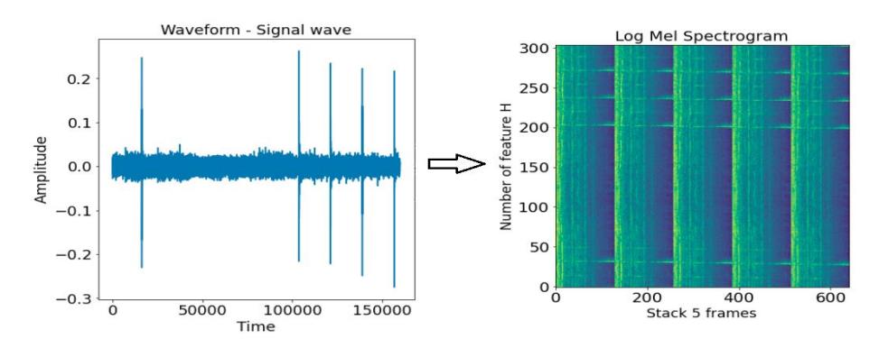
Figure 1 The waveform is converted to the log-Mel spectrogram feature.
We use 304 as the batch size in training and 640 as the 1D feature. Because the feature is created by being split into 5 frames and some machine type data has repeating patterns in the log-Mel spectrogram distribution, the log-Mel spectrogram is suitable to represent these types of machines.
2.1.2 The Mixed Feature
Based only on the log-Mel spectrogram, some important characteristics from the temporal domain may be missing from the feature space. The purpose of mixing different types of representations is to extract more information from the raw data. More information extraction leads to more coverage of the complex distribution of data. For example, for the machine type data in which there is no repeating pattern in the log-Mel spectrogram distribution, mixing different types of representations is more suitable. Acoustic features can be diverse, hardly following any repeating pattern. Based on the experimental results we selected five types of acoustic features to combine, which we call the Mixed Feature.
The Mixed Feature is a 1D vector constructed from five types of sound representations, i.e. MFCC, Chroma Feature, Mel Spectrogram, Spectral Contrast, and Tonnetz, respectively, as shown in Figure 2.
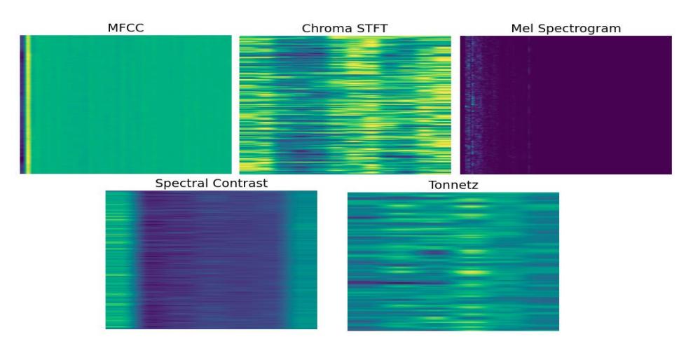
Figure 2 The five types of sound representations: MFCC, Chroma Feature (short-time Fourier transform), Mel Spectrogram, Spectral Contrast, and Tonnetz.
We chose these features based on their properties and to get more information from the sound so that we can better represent types of sounds with certain irregular distributions in the sound spectrum. We did not choose any more because the more time it takes to create these features, the more the latency in real-time prediction is increased. Corresponding to the frequencies in the Mel scale, we still keep the MFCC or the log-Mel spectrogram to combine with other feature types. We chose Chroma Feature because "identifying spectral components that differ by a musical octave, Chroma Feature show a high degree of invariance to variations in timbre and instrumentation while keeping their discriminative power" (Muller, et al. [11]). Spectral Contrast, "represents the relative spectral distribution instead of average spectral envelope. Spectral Contrast deals with the strength of spectral peaks, valleys, and their difference separately in each sub-band, and represents the relative spectral characteristics. Octave-based Spectral Contrast feature has a better discrimination among different music types than MFCC" (Dan-Ning, et al. [12]). As for Tonnetz, research into music cognition has demonstrated that the human brain uses a 'chart of the regions' to process tonal relationships (Wikipedia contributors in [13]).
- 1. We have 40 values from the mean of MFCC with the 40 cepstral coefficients.
- 2. We have 12 values from the mean of Chroma Feature by computing a chromagram from a power spectrogram (short-time Fourier transform).
- 3. We have 128 values from the mean of Mel Spectrogram by computing a Melscale spectrogram.
- 4. We have 7 values from the mean of Spectral Contrast by computing spectral contrast from a power spectrogram.
- 5. We have 6 values from the mean of Tonnetz by computing the tonal centroid features.
The way to compute these five extracted feature types is shown in the feature extraction part of the Librosa library documentation [14]. All parameters were default.
Figure 3 shows the way in which the vector is constructed by average, after which these five extract feature types are stacked together. Therefore, each shape of the Mixed Feature is 1 x 193, is 1D with a 193 (40 + 12 + 128 + 7 + 6)-dimensional vector, which is then used as the input layer of the proposed method.
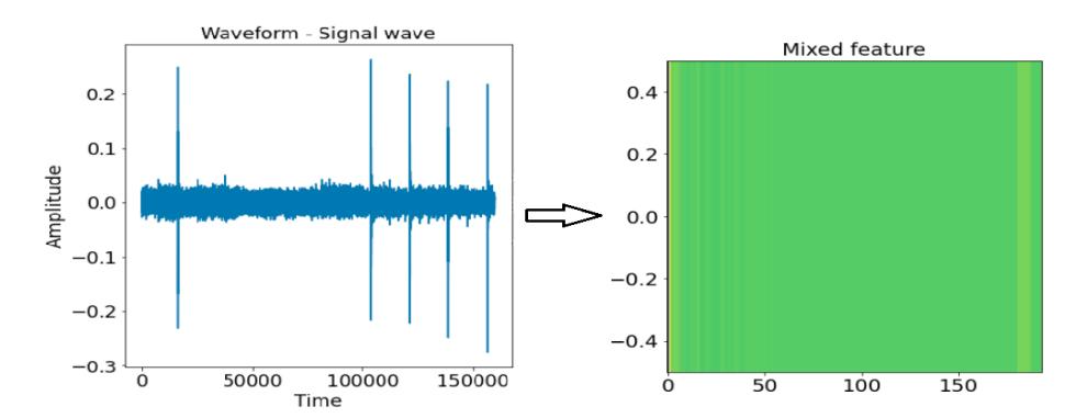
Figure 3 The waveform is converted into a new representation by average, stacking five types of features.
Figure 4 shows features of all machine types, respectively: ToyCar normal, ToyCar anomaly, ToyConveyor normal, ToyConveyor anomaly, Fan normal,
Fan anomaly, Pump normal, Pump anomaly, Slider normal, Slider anomaly, Valve normal, and Valve anomaly. The repeating patterns in the log-Mel spectrogram distribution are seen in Slider and Valve, whereas no repeating patterns occur in the log-Mel spectrogram distribution in ToyCar, ToyConveyor, Fan, and Pump. Therefore, the Log-Mel Spectrogram Feature was used for Slider and Valve, and the Mixed Feature was used for ToyCar, ToyConveyor, Fan, and Pump.
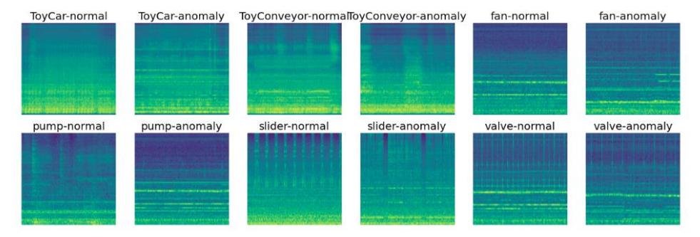
Figure 4 Log-Mel spectrogram of all machine types, respectively: ToyCar normal, ToyCar anomaly, ToyConveyor normal, ToyConveyor anomaly, Fan normal, Fan anomaly, Pump normal, Pump anomaly, Slider normal, Slider anomaly, Valve normal, Valve anomaly.
2.2 Fully Connected U-Net Architecture
Detecting abnormal sounds based only on normal sound samples is often used with autoencoder to produce the sound closest to the input sound for comparison with an anomalous sound. We still use the properties of the AE network. However, because we want to better keep information through layers, we apply the properties of the U-Net network given by Ronneberger, et al. [15]. However, the disadvantage of the original U-Net is that it can only work with twodimensional data.
The original U-Net uses convolution layers [16], which is very suitable in image data processing in order to reduce the number of hidden node units in the encoder and to increase the number of hidden nodes in the decoder. However, our data is sound and performs in 1D format. Our new proposed architecture, a fully connected architecture based on the original U-Net called Fully Connected U-Net, solves this problem by replacing convolution layers with dense/fullyconnected layers. Our new architecture inherits the benefits of keeping information from the encoder to the decoder to minimize the reconstruction error in normal data. In short, Fully Connected U-Net performs better because this architecture uses a fully connected layer instead of the convolutional layer in the original U-Net.
Dense/fully connected layers have the same formulas as linear layers ∗ + , but the end result is passed through a nonlinear function called the activation function, as shown in Eq. (1):
\[y = f(w * x + b) \tag{1}\] where is the input, is the output, is the weight, is bias and is a nonlinear activation function.
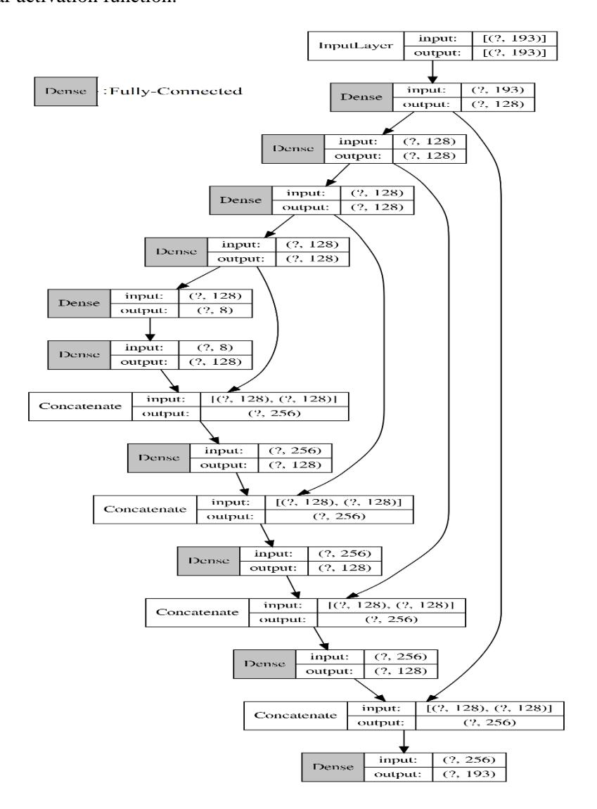
Figure 5 Fully-connected U-Net architecture.
Figure 5 shows the architecture with U-Net formed in a fully-connected structure. The architecture looks like a 'U', hence its name.
The architecture consists of three sections: the contraction section, the bottleneck section, and the expansion section. The contraction section consists of many contraction blocks. The number of kernels or feature maps after each block doubles so that the architecture can learn complex structures effectively. The bottleneck layer lies between the contraction layer and the expansion layer. The structure and number of units for each hidden layer is the same as the baseline auto-encoder from Koizumi, et al. [10], but Fully Connected U-Net uses concatenate layers to contract between pairs of layers in the encoder and decoder. The concatenate layer is the most significant part of this model because a lot of information is still kept from the encoder to the decoder. This is a strong novelty of the proposed method.
3 Experiment Settings
In our experiments, we used the Toy ADMOS from Koizumi, et al. [17] and the MIMII Dataset from Purohit, et al. [18] consisting of normal/anomalous operating sounds of six types of toys/real machines. Each recording is a singlechannel, 10-second long audio that includes both the target machine's operating sound and environmental noise.
The following six types of toys/real machines were used: ToyCar (Toy ADMOS), ToyConveyor (Toy ADMOS), Fan (MIMII Dataset), Pump (MIMII Dataset), Slider (MIMII Dataset), and Valve (MIMII Dataset).
Our experimental results were used to compare with the result of the baseline system. The baseline system is the simple autoencoder-based anomaly score calculator from Koizumi, et al. [10]. The anomaly score is calculated as the reconstruction error of the observed sound. To obtain small anomaly scores for normal sounds, the autoencoder architecture was trained to minimize the reconstruction error of the normal training data.
We used only the development dataset, with a 90/10 train/validation split. To reduce the learning rate when a metric has stopped improving, we used the Reduce LR On Plateau method, developed at Google by the Keras team in [19] with a factor of 0.5, a minimum learning rate of 10−4 , and patience 30. We also used the early stopping method with patience 50 for stop training when a metric stopped improving after 50 epochs. We trained 10,000 epochs, with a batch size of 512, and the Adam optimizer with a learning rate of 10−3 . The loss function for all methods was the default mean square error (MSE) as expressed in Eq. (2):
\[MSE = \frac{1}{n} \sum_{i=1}^{n} (Y_i - \underline{Y}_i)^2\] (2)
where n is the number of data points in a single batch, Y is the observed value, and \(\underline{Y}\) is the predicted value.
4 Results
Figure 6 shows the five frames in the log-Mel spectrogram concatenated together. Regarding the error difference between the original input and the reconstruction (error = input - reconstruction), we can observe the bold dots on the error of Valve's anomaly data more clearly than on the error of Valve's normal data. This shows that the loss value of the anomaly data is higher than the loss value of the normal data.
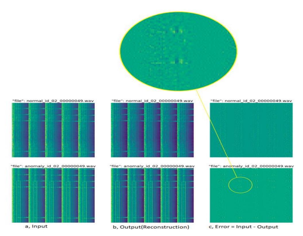
Figure 6 Comparison between input, output (reconstruction), error for the log-Mel spectrogram of Valve.
Figure 7 shows the Mixed Feature, which contains much information from the raw data.
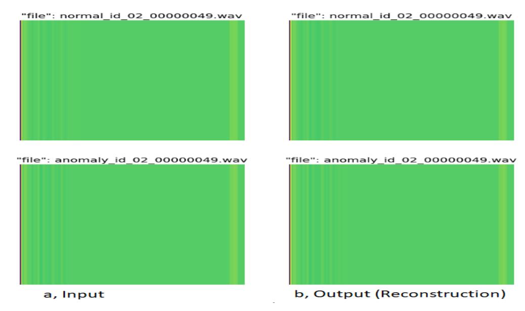
Figure 7 Comparison between input and reconstruction from the Mixed Feature of Valve.
Our target was to minimize the reconstruction error of the normal data. Based on experimentation, the loss value of our proposed method was lower than the loss value of the baseline system with a corresponding ratio of 4 and 10.
For this task, the evaluation metrics used is the area under the receiver operating characteristic (ROC) curve (AUC) and the partial-AUC (pAUC). The AUC and pAUC are defined in Eq. (3) and Eq. (4):
\[AUC = \frac{1}{N_{N_i}} \sum_{i=1}^{N_-} \sum_{j=1}^{N_+} H(A_{\theta}(x_j^+) - A_{\theta}(x_i^-))\] (3)
\[AUC = \frac{1}{N_{-}N_{+}} \sum_{i=1}^{N_{-}} \sum_{j=1}^{N_{+}} H(A_{\theta}(x_{j}^{+}) - A_{\theta}(x_{i}^{-}))\] \[pAUC = \frac{1}{|pN_{-}|N_{+}} \sum_{i=1}^{|pN_{-}|} \sum_{j=1}^{N_{+}} H(A_{\theta}(x_{j}^{+}) - A_{\theta}(x_{i}^{-}))\] \[(3)\]
The pAUC is derived from the AUC, calculated from a portion of the ROC curve over a pre-specified range of interest. In our metric, the pAUC is calculated as the AUC over a low false-positive-rate (FPR) range [0, p] with p = 0.1, from Koizumi et al. [10].
The AUC in Figure 8 shows that Fully Connected U-Net outperformed the autoencoder architecture from the baseline system taken from [10].
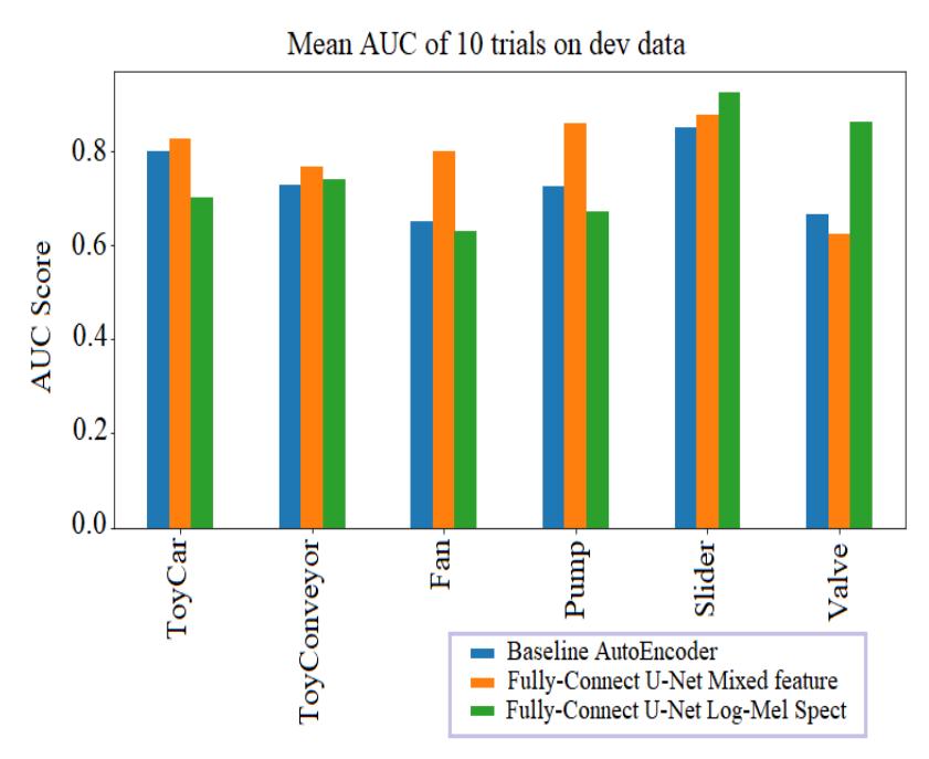
Figure 8 Mean AUC of 10 trials on every machine.
Fully Connected U-Net using the Mixed Feature was effective towards the ToyCar, ToyConveyor, Fan, Pump, and Slider machine types. Using the Mixed Feature, we observed the most improved results from Fan and Pump machine types. Fully Connected U-Net using the Log-Mel Spectrogram Feature was effective towards the Slider and Valve machine types. Fully Connected U-Net using the Log-Mel Spectrogram Feature for the Slider and Valve machine types helped to improve the average score of all machine types, such as AUC from 79.20 to 83.38, and pAUC from 61.50 to 64.51. Using only the Mixed Feature still outperformed the baseline system. For optimal results, we used the Log-Mel Spectrogram Feature for the Slider and Valve machine types, and Mixed Feature for the ToyCar, ToyConveyor, Fan, and Pump.
The AUC and pAUC were evaluated using GTX 1080 Tion the development dataset. Because the results produced with a GPU are generally nondeterministic, to simulate the same experiments as the baseline system, we also averaged 10 independent trials in training and testing. The experimental results for the means of 10 trials are shown in the following Table 1. This table shows that conventional U-Net and other CNN structures (WaveNet, LSTM) did not perform well, either underfitting or overfitting. All AUC and pAUC scores of our methods were higher than the AUC and pAUC scores of other methods from the literature (AE, IDNN).
| Mean AUC | Mean pAUC | |||||||
|---|---|---|---|---|---|---|---|---|
| Machine Type | Base line | Wave Net | UNet | LSTM | IDNN | Proposed | Base line | Proposed |
| ToyCar | 78.77 | 59.43 | 44.60 | 58.81 | 73.92 | 82.52 | 67.58 | 66.34 |
| ToyConveyor | 72.53 | 66.09 | 46.35 | 52.85 | 77.00 | 76.75 | 60.43 | 55.65 |
| Fan | 65.83 | 51.34 | 50.77 | 51.27 | 70.74 | 80.06 | 52.45 | 58.61 |
| Pump | 72.89 | 61.57 | 31.04 | 62.36 | 75.44 | 85.97 | 59.99 | 71.10 |
| Slider | 84.76 | 61.34 | 31.48 | 61.49 | 90.42 | 90.13 | 66.53 | 73.97 |
| Valve | 66.28 | 55.45 | 49.12 | 48.14 | 92.52 | 84.87 | 50.98 | 61.38 |
| Average | 73.51 | 59.03 | 42.22 | 55.82 | 80.80 | 83.38 | 59.66 | 64.51 |
Table 1 Experimental results for the means of 10 independent trials.
5 Conclusion
In this paper, we proposed methods to detect anomalies in sounds from machines. The proposed methods were applied to normal datasets without abnormal data. The contributions of this paper are as follows:
- 1. Propose and evaluate the Mixed Feature for data with no repeating patterns in the log-Mel spectrogram distribution.
- 2. Propose the Fully Connected U-Net architecture, a single model effective for all types of machine data for anomaly detection tasks.
The experimental results verified that our methods performed better than the baseline system. With the same model architecture and all hyperparameters fixed, our model achieved 83.38% AUC and 64.51% pAUC on average overall machine types provided with the developed dataset and outperformed the published baseline by 13.43% AUC and 8.13% pAUC.
In the future, we plan to enhance training using data augmentation. We will continue to develop algorithms that can detect more types of complex sounds, and we will tackle the remaining anomaly detection issues with the sound systems in real environments.
Acknowledgement
This work was supported by FPT Software AI Committee, FPT Software Company Limited, Hanoi, Vietnam. We also thank the anonymous reviewers for their careful reading of our paper and their insightful comments.