
1 Introduction
Wireless sensor networks can contain hundreds or more collaborative sensor nodes that are connected to each other. Sensor nodes are low-cost, easy-to-move, and light-weight devices that contain a microcomputer, energy source, transceiver, and transducer to produce electrical radar. However, these nodes have limited capacity and energy as they rely on limited energy sources (batteries) [1,2]. Most of the time, the surrounding environment of the sensors presents an obstacle to recharging or replacing their batteries. Therefore, reducing energy consumption is important to extend and improve the lifetime of WSNs, thus improving their performance and productivity [3]. To that end, different types of clustering algorithms and techniques have been proposed, for example hierarchical, distributed, and centralized techniques.
Clustering is a method used for grouping sensor nodes into clusters with a cluster head (CH) that is responsible for receiving data from its nodes members and forwarding them to the sink, or base station (BS) [4]. The CH has the smallest distance from the sink, the maximum number of neighboring nodes, and higher energy use than the other nodes. The CH uses a data aggregation function that helps in reducing the cost of transmission and removes redundancy [5]. Such protocols are widely used for large WSNs, for example, Low-Energy Adaptive
Received February 10th, 2021, 1st Revision April 27th, 2021, 2nd Revision June 1st, 2021, Accepted for publication July 21st, 2021.
Copyright © 2021 Published by IRCS-ITB, ISSN: 2337-5787, DOI: 10.5614/itbj.ict.res.appl.2021.15.2.5
Clustering Hierarchy (LEACH), and Power Efficient Gathering In Sensor Information Systems (PEGASIS). It is well established that efficient energy routing algorithms play a vital role in developing WSNs [6].
In this paper we propose several models to reduce power consumption in WSNs. We worked on the structure of the network, use the data transfer mechanisms, and choose the shortest routing path for data transmission between the sensor nodes and the sink. To test our proposed models, we performed comprehensive experiments and comparisons, including two scenarios for the location of the CH. A novelty of this paper is the proposal of a dynamic CH selection method. In this method, the CH is initially positioned at the center of the cluster and then repositioned at different stages of the network lifetime based on its distance from low-energy sensor nodes in the cluster. This dynamicity solves the overlapping coverage between sensor nodes in clusters and unbalanced energy consumption in the network, and leads to reduced network energy consumption and increased network lifetime.
The rest of this paper is organized as follows. In Section 2 we give a brief background and related work. Power consumption concepts and routing protocols are discussed in Section 3. We present our research methodology and experiment settings in Sections 4 and 5 respectively. In Section 6 we discuss the results, and we conclude the paper in Section 7.
2 Background and Related works
A wireless sensor network is a collection of low-power, low-cost, tiny, lightweight and easily removable devices known as sensor nodes. Each node consists of a transceiver, a transducer, a micro-controller, and an energy source [7].
In WSNs, sensors are randomly set up with limited power. Sensor nodes are energy constrained, where recharging or replacing the battery is an expensive and complex process. Therefore it is crucial to find solutions to reduce energy consumption, and extending and improving the network's lifetime [8]. One key solution is the use of clustering methods with an energy-efficient routing protocol that chooses the optimal CH with minimum transmission and energy costs [9].
Locating the optimal CH solves the overlapping coverage between sensor nodes in clusters and unbalanced energy consumption in the network. The authors of [10] presented DCHSM, which is a dynamic CH selection method. Another selection method is based on the distance from low-energy sensors, creating a balance between clusters [11]. The static cluster and dynamic cluster head mechanisms (SCDCH) proposed by [12] estimate the path of any transmission in an environment with minimum energy. Meanwhile, [13] used the nearest sensor position from the target to be the approximate position of the target's actual location. In [14], the Energy Efficient Clustering Scheme (EECS) is presented, which is a fully distributed and load-balanced clustering scheme. In EECS the network is partitioned into a set of clusters. Each set has one localized CH and without iteration connects directly with the BS, without intermediate nodes (single-hop). iLeach, proposed in [15], uses randomization to equally distribute energy among the sensors in a network. A new algorithm was developed to calculate the optimal probability to choose a node to become a CH in order to reduce energy consumption. PEGASIS was used by [16] in the field of environmental monitoring systems to handle energy consumption problems in different scenarios. The sensor node scenarios were divided into static and random. The fixed sink scenarios were: positioned in the middle of the network, outside the network, and in a corner of the network. Ref. [17] compares the wellknown protocols LEACH and PEGASIS in a wired and a wireless sensor network system on several different aspects, such as various package sizes and data transfer capabilities.
3 Routing Protocols
The authors of [18] and [19] proposed a centralized routing protocol for basestation control, called BCDCP, to improve average energy savings using a dynamic clustering protocol and to prolong network lifetime. BCDCP uses a high-energy BS because of energy-intensive tasks such as setting up clusters, routing paths, and performs randomized rotation of cluster heads.
Cluster-based technology was used in a WSN to build a routing protocol that saves battery energy in sensor nodes and also increases network lifetime [20]. Energy harvesting techniques were used to slow down the energy consumption of the nodes. Wireless recharging was used as a solution to the battery's drainage problem, where the energy transfer task can be done by a mobile sink without human resources needed.
A hexagon-shape routing protocol using a clustering structures scheme to obtain network stability and overcome the energy consumption problem was used in [21]. The hexagon shape was used for random deployment of nodes, where cluster areas are divided into small seamless regions without overlapping in order to cover a large area and obtain full network coverage. These regions are called hexagons (cells).
The authors of [22] focused on in reducing the energy consumed when transmitting data to the BS from CH, by using a super cluster head (SCH). Ref.
[23] proposed six scenarios for WSN structures to reduce the energy consumed in large WSNs.
Power consumption in WSNs is classified in two ways. The first is good and useful consumption, and the other is negative consumption, which wastes energy. Useful consumption includes transmitting data, receiving data, forwarding queries to neighboring nodes, and query processing. Negative consumption includes idle listening, collision, packet control and overhearing, over-omitting, and transition [10]. Routing protocols designed for sensor nodes must be as energy-efficient as possible to extend network lifetime while ensuring good overall performance. The design of routing protocols is challenging and has many constraints and limitations, for example in terms of energy, storage and bandwidth at the central processing unit [9].
Hierarchical routing protocols are energy-efficient, where sensor nodes are grouped into clusters and a cluster head is elected for each cluster [24]. The cluster head gathers data from the other sensor nodes and routes data from the cluster to the next layer (next CH) or the BS. A hierarchical approach covers larger distances when data move from a lower clustered layer to a higher layer. This feature saves energy because the data reaches the BS faster [25].
4 Research Methodology
Since sensor nodes in WSNs have a huge amount of data to send to the BS, there should be a process that is helpful in collecting data in an efficient way because of the energy consumed by transmitting and receiving data when the WSN is an energy-constrained network. Data aggregation is a process in which sensor nodes collect data using aggregation to eliminate redundancy and thus to reduce energy consumption. Data aggregation techniques work to gather data in a way that reduces the consumed energy and prolongs the network's lifetime [26].
Dividing the WSN into clusters using a hexagonal shape, we investigated different options for the position of the CHs. We studied different scenarios for the communication between nodes to determine the best method. Finally, we used different cluster-based protocols in order to examine our proposed model and determined the best combinations of options. Network productivity, energy consumption, and the number of dead nodes were used as measures for evaluating the proposed method.
The sink is a special node that is the destination of all communication in the WSN, which already has aggregated data or sometimes may collect more data. Sink locations have an important effect on the energy consumption of the sensor nodes [27].
4.1 Data Aggregation
The nodes in a cluster can start to sense and collect data using their sensors and then transfer the data to the CH. Radio transmission of each node, except the CH, can be stopped until the node's role in the time slot allocated to it within the TDMA is scheduled again after receiving all data.
The CH aggregates data before sending it to the base node (aggregation). Therefore, TDMA scheduling preserves energy and increases the lifetime of the sensor nodes.
4.2 HEX WSN
Consider that N refers to the nodes that are distributed randomly in a specific area to monitor an environment and i refers to the node number, where n_1 is the i-th sensor node. There are 100 nodes in the network. Thus, the sensor nodes are called n_1, n_2, n_3…, n_100. Our HEX network model is shown in the Figure 1.
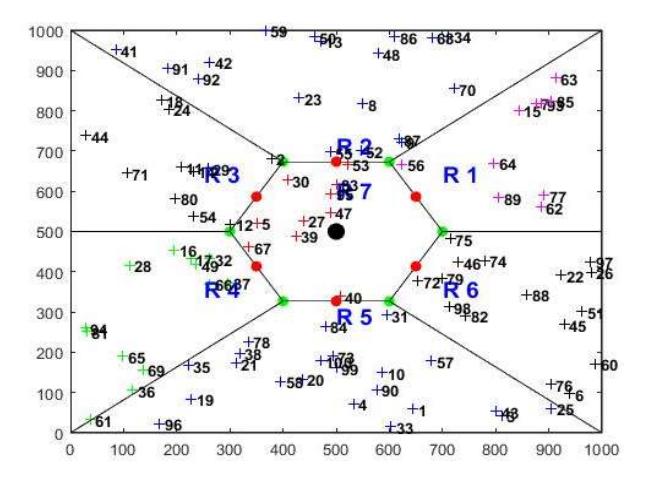
Figure 1 Static hexagonal WSN network.
To determine the path for the CHs we also used Dijkstra's algorithm. The simulation for proposed approach will be in MATLAB. We used a hexagonal shape for our wireless sensor network because it is comfortable and flexible; also it has a maximum coverage network sensor area [28]. The hexagram is the ideal form for the random distribution for sensor nodes in WSN because the clusters areas are smoothly divided by the HEX shape as shown in Figure 2. The hexagram covers the network area without overlaps and covers a larger area [21].
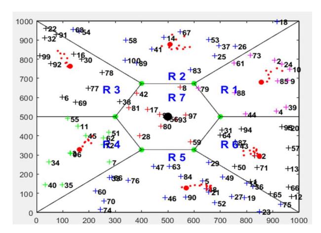
Figure 2 Dynamic WSN Hexagonal Network.
The CH used two scenarios for its position. One is called the static scenario, where the CH is fixed in the middle of each hexagonal side. The other one is called the dynamic scenario, where the CH moves to the middle position between all sensor nodes in its region using the arithmetic mean.
Each node in the network has coordinates (X, Y) that represent the location of the node. From this we find the arithmetic mean for all node coordinates in each region to move the CH to a suitable position in the middle of the nodes. Accordingly, the CH moves to this location, and when the first node dies, the CH changes its position again to fit and mediate the remaining nodes. The small red point in the dynamic CH in Figure 4 indicates the central position of the CH after some nodes have started to die. A dynamic CH helps in reducing the time and distance for a large number of nodes in terms of data transmission and communication with the CH, thus prolonging the lifetime of the network and saving energy.
4.3 Initial Phase
We used identical sensor nodes deployed randomly in the network, as shown in Figures 3 and 4. The sink transmits packets of size 4000 bits to the sensor nodes, and all nodes in the network are responding by sending their location and information to the sink or to the CH. The location of the CH will be explained later. The location of the sink is in the center of the network.
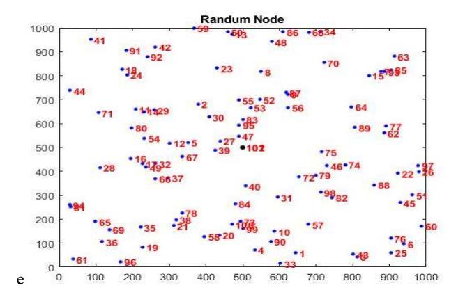
Figure 3 Random distribution of 100 nodes.
The CHs aggregate the data that comes from the nodes in their cluster and sends it to the sink. The sink has a table for collecting data received from all sensor nodes in the network. The data include the location of the node, the residual energy for each sensor node, the node ID, and the distance from the node to the CH and the sink.
4.4 Setup Phase
We divided the network area into seven logical regions according to the location of the node in the network (one inside the HEX shape, six regions outside the HEX shape). The outside six regions were divided according to the angles of the hexagonal. Each region is called a cluster. Each cluster has a CH, except the central cluster (region inside the HEX shape). Each CH has high energy.
The sink receives data in two ways: (1) directly, and (2) indirectly. For direct reception: sensor nodes in the central cluster aggregate their data and transfer it directly to the sink. Indirect transmission data occurs when a sensor node transfers its data to another sensor node that will eventually transfer it to the sink.
For the other clusters, the sensor node will transfer its data to the corresponding CH (direct and indirect). For a specific sensor node, the corresponding CH is the CH of the cluster that the node belongs to. The CH aggregates data and forward them to the sink. Finally, sensor nodes that are far away from the CH communicate with the closest node to reach its in-charge CH.
As mentioned earlier, the CH has two cases: fixed and moving. In the moving CH case, we assume it is mobile, for which we give the CHs high energy to do their job. CHs are created for every region separately, where each CH is responsible for a group of sensor nodes. The CH is an external node and is not considered a common sensor node in the network, i.e. a CH has relatively high-level energy, unlike sensor nodes. Moreover, dynamic CHs have the ability to be mobile (a CH can move from one place to another as we will explain when discussing the dynamic type).
To move from one location to another we assume that the CH is attached to a moving robot. In our network, we have six CHs for each region (cluster). The CH energy is calculated with the following Eq. (1):
\[ECH = (1 + a) * E0\] (1)
where, E0 is the initial energy of normal nodes, a is a constant, and the CHs have E0(1 + α) energy.
Dijkstra's algorithm, or Dijkstra's Shortest Path First algorithm, is an algorithm that finds the shortest path or best path between nodes to reach a destination, whether its is a CH or a sink, with the least possible cost. Dijkstra's algorithm is commonly applied in routing; it creates a tree of all the shortest paths with a nonnegative cost for each edge between nodes. Dijkstra's algorithm is stopped when it reaches the target, which is the minimum cost path between two nodes.
4.5 Illustration of the Study
Figure 4 summarizes the main steps of our proposed approach in a simple flowchart. From these cases we have four models for comparison in our paper:
- 1. Static Cluster-Based. In this model we use cluster-based communication with static location of the CH. The CH is fixed in the middle of each hexagonal side of the network shape. The communication between the sensor nodes and the CH or BS is direct, where the nodes send the data they collected from the sensing area to the CH directly without intermediate node.
- 2. Dynamic Cluster-Based. In this model we use cluster-based communication with dynamic location of the CH. The CH moves to the middle position between groups of sensor nodes. Upon the death of his first sensor nodes, the CH changes its position to mediate the remainder of the sensor nodes in the area for which it is responsible. This transition is done by using the mean of the sensor node locations in each region. The communication between the sensor nodes and the CH or BS is direct, where the nodes send the data they collected from the sensing area to the CH directly without intermediate node.
- 3. Static Chain-Based. In this model we use chain-based communication with static location of the CH. The CH is fixed in the middle of each hexagonal side of the network shape. The communication between the sensor nodes and the CH or BS is as a bus or chain from all nodes in the cluster to the CH or BS.
4. Dynamic Chain-Based. In this model we use chain-based communication with dynamic location of the CH. The CH moves to the middle position between the sensor nodes. Upon the death of the first sensor nodes, the CH changes its position to mediate the remainder of the sensor nodes in the area for which it is responsible. The communication between the sensor nodes and the CH or BS is as a bus or chain from all nodes in the cluster to the CH or BS.
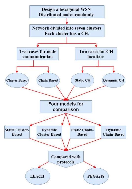
Figure 4 The proposed approach.
5 Experiment Settings and Parameters
We simulated the proposed approach using (MATLAB). We used a network of 1,000 m x 1,000 m with 100 random nodes spread in the network. The sink position was at the center of the sensing field, and the CH position was in the middle of the hexagonal sides. After node dissemination, the sink and CHs stayed fixed in their positions. The packet size used was 4,000 bits. We compared our approach with the LEACH and PEGASIS protocols on several aspects, such as consumed energy, number of dead nodes, and number of packets (we did not take into account the consequences of collision or interference of wireless channels in evaluating the performance, according to [23]). Table 1 presents the parameters of our simulation.
Parameters Values 1,000 m x 1,000 m Network area Number nodes 100 nodes Number of WSN rounds 3,000 rounds Data packet size 4.000 bits Transfer energy ETx = 50*0.000000001Receive energy Erx = 50*0.000000001Initial energy 0.5 joule (500,500)Sink position
Table 1 Simulation parameters.
We evaluated our simulation based on the following three network performance criteria:
- 1. Network lifetime: the time that the network operated, which is defined as the network uptime during which it can perform its specific tasks [29].
- 2. Throughput: the total number of packets that were sent to the sink or cluster heads during the network lifetime [30].
- 3. Residual energy: the average remaining battery energy for active sensor nodes in the network at the end of each simulation experiment. Residual energy is used for study and analysis of the amount of energy that the sensor nodes consumed in each round [31].
Eq. (2) [23,32] shows the calculation of the energy consumed when transmitting a packet consisting of k-bits over a transmission distance of \(E_{Tx}\) (k, d).
\[E_{Tx}(k, d) = E_{elec} *k + Camp *k * d^2, d > 1\] (2)
where k is the data volume that has to be transmitted, d is the distance between the two nodes. \(E_{\rm elec}\) is the energy used to take out the data transmission in terms of nJ/bit.
Eq. (3) shows the average energy consumption, E, referring to the average energy consumed by a successfully transmitted packet [33]. It can be expressed as:
\[E_{average} = \frac{Total energy consumed}{Number of packets received}\] (3)
6 Results and Discussion
In this section, we present our results and discuss them. We divide this section into two subsections. In the first subsection we compare our four proposed models to decide on a 'winner' among them, while in the second subsection we compare our winner to PEGASIS and LEACH.
6.1 Deciding on a Winner
In order to specify the best model among our four proposed models, i.e. the winner, we compare them according to the following three categories.
6.1.1 Dead Nodes
As can be seen in Figure 5, the percentage of total dead nodes for the Static Cluster-Based model for 100 nodes after 3,000 rounds was 95%. For the Dynamic Cluster-Based model, the percentage of total dead nodes for 100 nodes after 3,000 rounds was 86%. For the Static Chain-Based Model, the percentage of total dead nodes for 100 nodes after 3,000 rounds was 88%. Finally, for the Dynamic Chain-Based model, the percentage of total dead nodes for 100 nodes after 3,000 rounds was 81%.
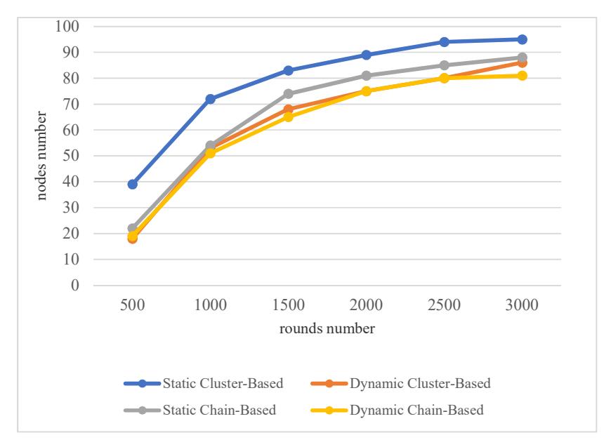
Figure 5 Average dead nodes.
6.1.2 Consumed Energy
Figure 6 shows the average of consumed energy. The total energy consumed by the network with 100 sensor nodes was 0.5 joules. The total energy consumed for transmitting data for the Static Cluster-Based model was 49.308 and the percentage of energy consumption was 98%. For the Dynamic Cluster-Based model it was 47.924 and the percentage of energy consumption was 95%. For the Static Chain-Based model it was 48.162 and the percentage of energy consumption was 96%. For the Dynamic Chain-Based model it was 43.849 and the percentage of energy consumption was 87%.
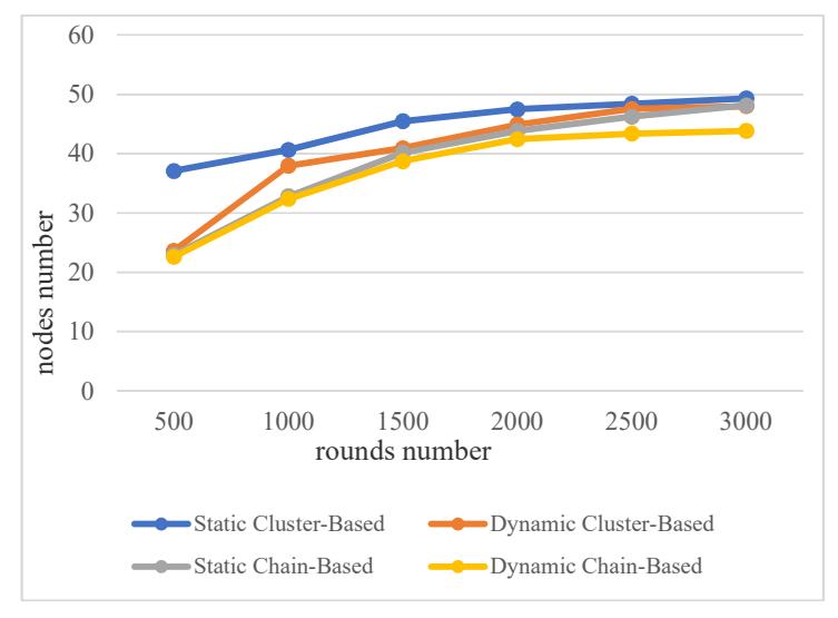
Figure 6 Average consumed energy.
6.1.3 Transmitted Packets
Figure 7 shows that the total number of packets that were transmitted for the Static Cluster-Based model was 71,038 packets and the average percentage of sent packets/round was 23.7%. For the Dynamic Cluster-Based model the total number of packets was 123,819 packets and the average percentage of sent packets/round was 41.2%. For the Static Chain-Based model the total number of packets was 107,999 and the average percentage of sent packets per round was 36.0%. For the Dynamic Chain-Based model the number of packets was 130,535 packets and the average percentage of sent packets per round was 43.5%.
As for the previous comparisons, it is obvious that the Dynamic Chain-Based model outperformed the other proposed models. We believe that this is due to the fact that having a dynamic CH that moves according to the evolution of the network and therefore gets closer to the remaining low-energy nodes will reduce their power consumption, thus increasing their life time and decreasing the number of dead nodes.
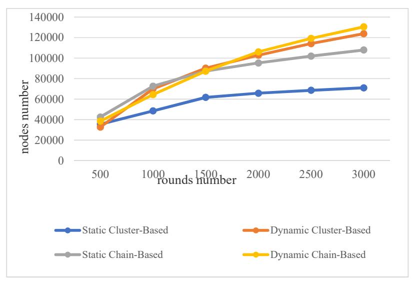
Figure 7 Average packet nodes.
6.2 Comparison with Well-known Protocols
In this subsection, we compare our winner, i.e. the Dynamic Chain-Based model, with the two main routing protocols, LEACH and PEGASIS. LEACH uses cluster-based clustering and PEGASIS uses chain-based clustering. We performed these comparisons based on the same three factors that we used in the previous comparisons. We relied on the results reported in [23].
6.2.1 Dead Nodes
In LEACH, 100 nodes were dead before 1,500 rounds were completed. In PEGASIS, 100 nodes were dead before 2,500 rounds were completed. However, our proposed model completed 3,000 rounds and all nodes were still alive; this is because the HEX was divided into logical clusters, where each one had a CH and energy stabilization within the sensor nodes. As can be seen from Figure 8, the number of dead nodes and the distribution of dead nodes during the HEX rounds was better than for LEACH and PEGASIS. This is because of the good distribution of energy within the sensor nodes. Thus, our model topology had the longest lifespan.
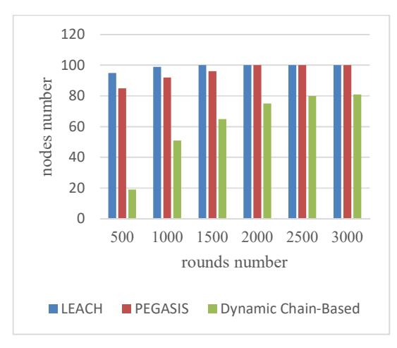
Figure 8 Dead node comparison.
6.2.2 Consumed Energy
Figure 9 shows that the amount of energy used for each round was less for our proposed protocol compared to LEACH and PEGASIS. The best result in energy consumption was for our proposed model (87%), followed by PEGASIS, which consumed 100% energy before round 2500, and LEACH, which consumed 100% energy before 1500 rounds. Our protocol guarantees the use of the least amount of energy. This is due to the dissemination of the sink at the center of HEX. Moreover, the CHs in all clusters help in reducing energy consumption and extend the network's lifetime.
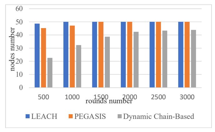
Figure 9 Energy consumption.
6.2.3 Transmitted Packets
Figure 10 shows that the total number of packets transmitted using LEACH was 2,254 and the average percentage of sent packets/round was 0.8%. For PEGASIS the total number of packets transmitted was 13,042 and the average percentage of sent packets/round was 4.3%. In our proposed model the total number of packets transmitted was 130,535 and the average percentage of sent packets/round was 43.5%.
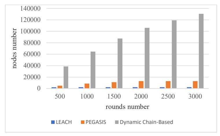
Figure 10 Total number of packets sent comparison.
7 Conclusion
The most common problem facing WSNs is the limited power in their devices, where the capacity of the batteries used in the sensors is limited. The question is always how to deal with energy consumption problems and the network design in a way that guarantees a prolonged lifetime.
In this paper, we proposed a hexagonal model for WSNs. The network is divided into seven zones. The sensor nodes are distributed randomly in a HEX shape network. There are six CHs, which are installed in the middle of each hexagonal side. The sink is located in the center of the HEX network.
We studied four cases on a hexagonal grid and its effect on extending the network life and reducing its energy consumption. Our network had an estimated energy consumption of 50 joules. The result of energy consumption in the previous cases was as follows: the best result was for the Dynamic Chain-Based model, where the percentage of energy consumption was 88%, followed by the Dynamic
Cluster-Based model with a rate of 95%, then the Static Chain-Based model with a rate of 97%, and finally the Static Cluster-Based model with a rate of 98%.
Our approach performed better than the PEGASIS and LEACH protocols, where energy consumption was 100%. Our proposed model also had the best results in terms of the largest number of packets transmitted in the network utilizing the available energy to achieve maximum efficiency of the network. In addition, the network completed 3,000 rounds and was still alive, unlike PEGASIS and LEACH, which ended the network's life before the completion of 2,000 rounds. The comparison demonstrated the superiority of the proposed model as is increased the average number of living nodes after 3,000 rounds of the network by 19%.