
1 Introduction
Malware is defined as intrusive software that penetrates or destroys a system without permission of the user. Malware is a common concept that threatens all sorts of devices. A basic malware distinction is between file infectors and individual malware. According to the specific behavior malware items can be classified into adware, viruses, trojans, spyware, rootkits, etc. The process of malware detection through traditional signature-based methods (Santos, et al. [1]) is very problematic because all older and new malware programs have polymorphic layers to avoid detection; the use of lateral mechanisms assists in developing new malware versions in a shorter time in order to avoid antivirus detection. For malware identification through dynamic file review in a virtual
world, the interested reader is referred to Rieck et al. [2]. The classical methods for detecting metamorphic viruses are discussed in Konstantinou, et al. [3].
Cyber threats become possible when criminals use malware as a primary weapon in their operations. Therefore, one information protection issue is to detect ransomware in time so that it can be blocked to prevent the attackers from accomplishing their goals, or at least delay them long enough to stop them.Various detection methods, such as regulatory or signature-based methods, enable the analyst to apply rules manually based on specific data to identify and automatically describe harmful or sensitive data to the specifications of the detection model. The automated generation of signatures is a middle ground between these two methods. To date, manual and automated rules and signatures have been used in the information security field using machine learning and mathematical techniques due to the low false positive rates they can achieve.
In recent years, however, three advances have strengthened the potential for progress in machine-based learning techniques, suggesting that these strategies will attain high detection rates at low false positive rates without the pressure of producing manual signatures. The first such trend is the rise of commercial threat intelligence feeds that offer large quantities of new malware, which means that the safety community has access to labeled malware for the first time. The second trend is that processing power has become cheaper, so researchers can travel more easily around learning models in malware detection systems and fit larger and more complex models to the results. Thirdly, machine learning has developed as a discipline, which means that researchers have more resources for effective detection models that can achieve both accuracy and scalability breakthroughs.
1.1 Motivation of the Study
Malware (such as viruses, trojans, ransomware, and bots) pose substantial emerging security risks to Internet users. Anti-malware security services from a variety of firms, including Comodo, Kaspersky, Kingsoft, and Symantec, offer primary protection against malware. To keep up with the growing number of malware items, intelligent methods for accurate and reliable malware identification from large everyday sample collections are urgently needed. This research first provides a brief introduction about malware, types of malware and the need for malware detection using machine-learning techniques. In these methods, the process of detection is usually divided into two stages: feature extraction and classification. The result is subjected to malware detection by five different classifiers that are used in the decision making process and among those the best output is selected.
1.2 Malware
Malware is software that is used or designed to interrupt network processes, capture personal information, or control private computer systems. It can be found in JavaScript, scripts, active content, and applications. Malware is commonly used as a term to refer to several types of software that is offensive, disruptive, or irritating.
Malware Use:
- 1. Many early infectious programs were written as experiments or pranks, including the first Internet worm.
- 2. Today, malware is mostly used to capture confidential information for the benefit of others, including personal, financial and business information.
- 3. Malware is often used extensively to capture or destroy secured information from government or business websites.
- 4. Malware, however, is also used to obtain personal data such as credit card numbers, social security numbers, bank accounts etc.
1.3 Types of Malware
It is helpful to define malware and provide a clear understanding of the techniques and reasoning behind it. Depending on its intent, malware can be classified into several groups. The classes are the following:
- 1. Bugs This is the most simple software type. It is a single piece of software that starts excepting permission of the user when it is replicated, or other software is corrupted/modified (Horton [4]).
- 2. Worms This form of malware is pretty much like a virus, but a worm will spread to other devices across a network (Smith [5]).
- 3. Trojans This term is used to describe types of malware that are meant to function as legitimate applications. Moffie, et al. [6] explain that social engineering is the general spreading vector used in this field, which implies that people believe they are installing a legitimate application.
- 4. Adware The aim of this sort of malware is to display ads on a system. Adware is considered as a subset of spyware but is unlikely to lead to spectacular outcomes.
- 5. Spyware As the name suggests, this is malware that enables hacking. Typical spyware actions include monitoring of the user history to send targeted ads and follow behaviors to market them to mediators (Chien, et al. [7]).
- 6. Rootkit Its interface allows intruders higher authorization to access data on a system than is permissible. This may be used for example to provide illegal administrative user permission. Rootkits often mask their presence and are
- often unnoticeable on the device, rendering the identification and removal exceedingly difficult (Chuvakin, et al. [8]).
- 7. Backdoor This is a form of malware that allows attackers to access a device in an additional hidden fashion. It is not dangerous on its own but offers more room for attackers. As a result, backdoors are seldom used autonomously, they typically precede other forms of malware attacks.
- 8. Keylogger This malware is used to record all keys that are pressed by the user and store sensitive information such as card numbers and passwords (Chumachenk,o et al. [9]).
- 9. Malware This malware is intended to encipher all data on a device and force the target to send cash to obtain the decipher key. A ransom compromised system is normally 'frozen', so the user is unable to access any file. A screen image is used to supply data about the requests of the attacker (Savage, et al. [10]).
- 10. Remote Control Software (RAT) A RAT helps the intruders to enter a device and make changes to it as if they have physical access. It can be builtin but used with malicious motives, like in the example of TeamViewer.
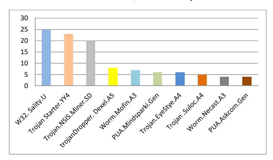
Figure 1 Top 10 Windows malware [30].
2 Methods of Detection
Malware identification approaches can be categorized into signatures-based and behavior-based strategies. It is crucial to consider the fundamentals of two malware analysis approaches before moving to the discussion of these methods: static analysis of malware, and dynamic analysis of malware. Static analysis takes
place 'statically', i.e. without processing any files. In contrast, dynamic file processing is carried out on a virtual machine.
Static research is interpreted as 'reading' the source code of malware and attempting to deduce behavioral features from the code. Various strategies can be used in static analyses (Prasad, Annangi & Pendyala [11]):
- 1. File format inspection: The file metadata can be helpful. For example Windows PE files contain information about time to compile, imported and exported functions, etc.
- 2. String extraction: This means program output inspection (for example, status or error messages) and the inference of malware process information.
- 3. Fingerprinting: This involves the calculation of the cryptographic hash, the identification of environmental items, including hard-coded usernames, passwords or strings in the registry.
- 4. AV scanning: If the examined file is known ransomware, it can possibly be found by all anti-virus scanners available. While this identification can seem insignificant, AV vendors or sandboxes use this identification tool to 'confirm' their results.
- 5. Disassembly: This involves the reverse of the program code to combine the language and structure and purpose of applications. This is the most widely used and accurate static analysis method.
- 6. Dynamic and static analysis: in contrast to static analysis, in dynamic analysis the file under investigation is tracked during execution and the features and purposes of the file are derived from these details. The file is normally run in a simulated environment, such as a sandbox. All behavioral characteristics such as opened directories, generated mutexes, etc. can be found during this method of analysis. It is also easier compared to static analysis. Static analysis only reveals the behavioral situation that is applicable to the present device characteristics. If a virtual machine is built under Windows 7, then the results may vary from those of Windows 8.1 malware (Egele, et al. [12]).
One form of static analysis is called signature-based analysis and is based on pre-defined signatures, which may be fingerprints, static strings, SHA1 or MD5 hash, or metadata tabs. The identification condition will be the following: when a file appears on a device, the anti-virus program analyzes it statically. If one of the signatures matches, an alarm is activated such as 'This file is suspect'. Most frequently this analysis method is appropriate and familiar malware samples are also found based on hash values.
2.1 The Need for Machine Learning
In the past decade, the study and the use of machine-learning tools have expanded to solving tasks of malware identification and classification. Fig. 2 depicts the machine-learning workflow of malware detection. Without the confluence of three recent innovations, the progress and convergence of machine-learning methods would not have been possible:
- 1. The first change is a spike in malware feeds, which means that for the first time branded malware is not only available in the defense area but also in the testing area. The size of this feed varies from small top-quality specimens, such as those provided by Microsoft [13], to vast quantities of malware, such as Zoo [14] and Chu [15].
- 2. Secondly, computing technology has grown exponentially and has become affordable and closer to the budgets of most researchers at the same time. As a result, researchers have improved the methods of iterative training and applied bigger and more complicated models and results.
- 3. Thirdly, the field of machine learning has advanced more quickly over recent decades, taking the precision and scalability of a variety of tasks such as device perception, natural language processing and speech recognition to new levels.
Signature-based malware detectors can do well with malware that has previously been detected by many anti-virus vendors. However, they cannot detect polymorphic malware that can modify its signatures or new malware, for which no signatures have been created yet. The sensitivity of heuristic detectors is not always sufficient to identify these correctly, resulting in numerous false positives and false negatives (Baskaran, et al. [16]).
The high distribution rate of polymorphic viruses dictates the need for modern detection methods. One solution to this problem is to focus on heuristic analysis combined with machine learning approaches that provide better detection results (Figure 2).
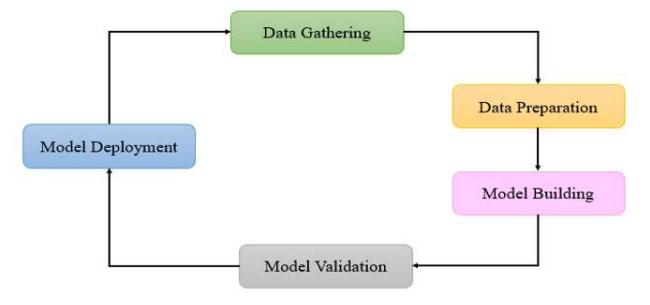
Figure 2 Machine learning workflow.
When using a heuristic process, there must be a certain level of malware activity, which determines the number of heuristics necessary to identify a program as malicious. For instance, a variety of suspicious operations such as 'changed registry key', 'link created', 'changed permit', etc., may be identified. It would also assume that every program that causes at least five of such operations may be considered malicious. While this strategy gives some degree of reliability, it is not necessarily valid, since there are features that may have extra 'weight' compared to others, for example, 'modified allowances' usually has more drastic effects on a device than 'adjusted registry key'. In comparison, certain combinations of features may be more questionable than the features separately (Rieck, et al. [17]).
3 Related Work
In 2001, Schultz, et al. [18] launched machine learning for finding new, staticbased malware, byte n-grams on program executables, and strings for functionality extraction writers. In 2007, Bilar [19] released Opcode, a malware finder to investigate the distribution of opcode frequency in non-malicious and malicious scripts. In 2007, Elovici, et al. [20] used Feature Range and Decision Tree (5 grams, top 300, FS), Bayesian Network (5 grams), Artificial Neural Network (5 grams, top 300, FS), Decision Tree (using the PE), BN (using the PE) and accuracy of 95.8 percent. In 2008, Moskovitch, et al. [21] used philtres for the collection of functions. For the collection and classification of functions and Decision Tree (DT), Naïve Bayes (NB), and Adaboost, Neural Support Networks (ANN). The assistance of support vector machine (SVM) and M1 (DT and NB boosted) using Fisher score and gain ratio (GR) had an accuracy of 94.9%.
Again, Moskovitch, et al. [22] used the n-gram (2,3,4,5,6 grams) of opcodes as standard and used the collection of document frequency (DF), GR and FS features in 2008. They used the ANN, DT, Boosted DT, NB and Boosted NB classification algorithms, which were outperformed by ANN, DT, BDT in retaining a low false positive score.
Santos, et al. [23] concluded in 2011 that supervised learning includes labeling data so that semi-controlled learning was introduced to recognize unknown malware. In 2011, the frequency of operating codes was again provided by Santos, et al. [24]. They used the function selection approach and various classifiers, i.e. DT, K-Closest Neighbors (KNN, Bayesian Network), Support Vector Machine (SVM) with an opcode sequence length of 92.92% and an opcode sequence length of 95.90%. Shabtai, et al. used n-gram opcode pattern features in 2012 to define the best available tool for document frequency (DF), G-mean and Fisher ranking. They used several classifiers in their method, with Random Forest exceeding 95.146% accuracy (Shabtai, et al. [25]).
In 2016, Ashu, et al. [26] proposed a new method for high-precision detection of unknown malware. They studied the frequency of opcodes and put them together. The authors tested thirteen classifiers, from which FT, J48, NBT, and Random Forest were included in the WEKA machine learning stage, and obtained over 96.28% accuracy for malware. In 2016, Sahay, et al. [27] using the Optimal K Means Clustering algorithm, clustered malware executables and these groups were used by classifiers to identify unknown malware as promising training features (FT, J48, NBT, and Random Forest). They found that the identification by the proposed solution of unknown malware had 99.11% accuracy.
Some scholars have recently been working on a new malware dataset for Kaggle [28]. In 2016, Ahmadi, et al. [29] collected Microsoft malware data and hex dump-based characteristics used (string length, metadata, entropy, n-gram, and image depiction) and also characteristics derived from unmounted files and the classification algorithms of XGBoost (metadata, icon duration, opcodes, registries, etc.). They achieved an accuracy of ~99.8%. For the 2017 classification of polymorphic malware, Drew, et al. [30] employed the Super Threaded Reference Free Alignment-Free N-sequence Decoder (STRAND) classifier. They introduced an ASM sequence model and achieved a precision of more than 98.59% with a 10-fold cross-validation approach.
In Souri, et al. [31], a number of malware detection techniques are presented in two categories:
- 1. signature-based methods, and
- 2. behavior-based methods. The survey, however, did not include either a study of the current deep learning methods or the types of features used for malware detection and classification in data-mining techniques. Ucci, et al. [32] categorized the methods according to:
- a. What is the objective problem they are trying to solve?
- b. What are the types of characteristics taken from portable executable files (PEs), and
- c. Which machine learning algorithms they use. Although the research provides a full overview of the taxonomy of functions, new research trends, notably multimodal and deep learning approaches, are not outlined.
Ye, et al. [33] cover common malware-detection machine-learning methods, consisting of the discovery, compilation and classification of items. However, core features like entropy or structural entropy and certain complex characteristics such as network operation, opcodes and API tracks are absent. In comparison, deep learning techniques or multimodal malware identification techniques are not included. Finally, Razak, et al. [34] have done a malware bibliometric study to examine publications related to malware by region, organization, and author. However, the paper does not define the features of malware detectors and does not consider the latest technologies in this field. Sakhnini, et al. (2019) [44] present a bibliometric survey focusing on the security aspects of IoT enabled smart grids. Furthermore, the authors address the problem of the different types of cyber attacks that they found related to a particular topic. Yazdinejad, et al. (2020) [45] designed a novel RNN model in order to detect malware threats in cryptocurrencies. The authors for this particular study collected 500 samples of cryptocurrency malware and 200 samples of goodware.
Table 1 Recent research in machine learning-based Android malware detection.
| Authors | Features | Algorithm | Comment |
|---|---|---|---|
| Sahs & Khan (2012) [46] | Permissions, CFG subgraphs | 1-class SVM | Sahs & Khan's approach yielded high recall with low precision. The vast majority of our in-lab classifiers yielded both a high recall and a high precision. |
| Amos, et al. (2013) [47] | Profiling (dynamic) | Random Forest, C4.5, etc. | Our closest experiment (goodware/ malware ratio: 1/2) yielded dozens of classifiers with equivalent or better performance. |
| Yerima, et al. (2013) [48] | API calls, external tool execution, permissions (static) | Bayesian | Our closest in-lab experiment (goodware/malware ratio: 1) yielded 74 classifiers with both higher recall and higher precision than Yerima, et al.'s best classifier. |
| Canfora, et al. (2013) [49] | SysCalls, permissions | C4.5, Random Forest, etc. | In our closest experiment by dataset size (good ware/malware ratio: 1/2), our worst classifier performed better than Canfora, et al.'s best classifier. In our closest experiment by good ware/malware ratio (1), the vast majority of our classifiers performed better than Canfora, et al.'s best classifier. |
| Wu, et al. (2012) [50] | Permissions, API calls, etc. | KNN, Naive Bayes | More than 100 of our in-lab classifiers yielded both a higher recall and a higher precision than Wu, et al.'s best classifier. |
3.1 Research Issues and Challenges
The following section discusses some of the problems and concerns that security scientists face.
- 1. Class imbalance: Collecting successful training data complicates aspects of any machine-learning problem. Machine-learning classifiers are as successful as the data they are fed to be qualified. Correctly labeling information is highly necessary to detect malware and can be a process that takes a lot of time.
- 2. Open and available benchmarks: The role of identifying and classifying malware is not the same as other programs with rich databases in the testing community. It includes digit scoring, voice recognition, photo labeling, etc. Legal limitations make this problem worse. Although web pages like VirusShare and VX Heaven openly distribute malware binaries, benign binaries are also protected by copyright laws from sharing. Nevertheless, benign and malicious binaries can only be accessed in bulk through providers such as VirusTotal for internal use, but subsequent distribution is forbidden.
- 3. Concept drift: The word 'concept drift' is used in the machine-learning literature to refer to the issue of interaction evolution in knowledge. Supervised learning is a function of the computer to transform an input to an output based on a series of input output samples. In technical terms, the problem is that the mapping function (f) given input data (x) is approximated in order to estimate an output (y), y = f(x). Common computer apps such as automated sorting, text categorization, or voice recognition presume that the data is taken from a population that is stationary. They believe that data mapped in the past will remain true in the future and that new data and the relations between input and output do not change over time. This does not extend to the issue of malware detection and classification.
- 4. Adversarial learning: Malware learns to live and function. In other words, malicious software must continuously improve in order to resist anti-malware detection. As a result, there is a strong incentive for malware authors to attempt to evade detection by using obscuring strategies (You, et al., 2010 [35]; O'Kane, et al., 2011 [36]).
- 5. Form interpretability: Understanding the latest available mechanical learning techniques is a problem (Shirataki & Yamaguchi, 2017[37]; Gilpin, et al., 2018 [38]). Many models being used are called a black box. A black box comes with an input X, which generates an output Y by a series of operations that are difficult for a human being to comprehend. This could pose a challenge when a false alert occurs in a cyber security application and researchers try to find out why it has occurred. The model's interpretability defines how quickly examiners can handle and analyze the output and correct the working of the defined model.
4 Materials and Method
We see malware analysis and identification as a binary classification problem, where the two types of software to be classified are malware and goodware.
Figure 3 shows that the proposed approach is a multi-step process consisting of various steps performing several tasks. The system can be divided into three parts: clustering, decision making, data processing, and dataset preparation and division.
4.1 System Architecture
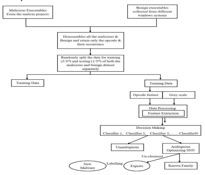
Figure 3 Block diagram of research methodology.
4.2 System Description
4.2.1 Description of Dataset
It is important to create a large dataset with several different samples to test the effectiveness of classical machine learning and deep learning architectures. Because of the privacy-preserving policies of individuals and organizations, publicly available databases for potential cyber security research for malware detection are extremely limited. Over time, the provision of one source for all kinds of malware families has become increasingly difficult as malware has evolved. Researchers share their findings, but all the necessary samples have not been collected in one single dataset or repository yet. In this study, the publicly accessible dataset Ember was used, with a subset containing 70,140 benign and 69,860 malicious files. This dataset was randomly divided into 60% training and 40% testing data using Scikit-learn. The training dataset consisted of 42,140 benign files and 41,860 malicious files. In the training dataset, 28,000 benign files and 28,000 malicious files existed. These samples were derived from VirusTotal, VirusShare and privately collected samples of benign and malware samples (Kaggle [28]).
4.2.2 Feature Extraction
As discussed above, our data kit consisted of 140,000 executable files. We disassembled these functions by translating the .exe file into an .asm file. The object dump tool that is part of the GNU Binutils package was used. When some executable files were disabled or encrypted, these files were deleted from the dataset.
4.2.3 Opcode n-gram
In order to reverse the malware review, we used IDA Pro. IDA Pro is a versatile dynamic disassembler published by Hex-Rays (Tian, et al. [39], Ye, et al. [40]). It is necessary to access the malware assembly code and use it to define function blocks and explain the process flow map, import methods, etc.
4.2.4 n-gram
In this analysis, we used an n-gram model to remove opcode functionality from the malware. It is an easy way to remove text functions. The presence of n terms is only correlated with the previous n − 1 terms, n being the length of one function sequence. If we have a set of L opcodes, then the set will be split into sequences of L – n + 1 attributes. This model seeks sequences of functions in a sliding pane. A 3-gram model, for example, is used to obtain functional sequences from for example, call, push, mov, add, pop, inc and xor. As shown in Figure 4, we take out five short strings, and three opcodes are used in each sequence.
| push | call | add | mov | xor | inc | pop |
|---|---|---|---|---|---|---|
| push | call | add | mov | xor | inc | pop |
| push | call | add | mov | xor | inc | pop |
| push | call | add | mov | xor | inc | pop |
| push | call | add | mov | xor | inc | pop |
Figure 4 Opcode 3-gram model
4.2.5 Feature Selection
Choosing features that can discern malware families is important. The features are extracted via the n-gram model as high-dimensional data. A modern approach is used to reduce the dimensionality of the data to increase classification accuracy and to minimize time usage. We discuss some definitions that aid in the definition. \(Y = \{0,1,...\}\) is the malware family, symbol \(S_i\) refers to a set of functions. The given Eq. (1) shows a frequency series:
\[f(s_i) = sum(s_i|y_i) / \sum_{isn_i} sum(s_i|y_i)\] (1)
where the number of the sequence belonging to family \(y_j\) is denoted by \(sum(s_i)\) and the frequency of the sequence in Y is \(F(s_i)\):
\[F(s_i) = \frac{\sum_{isn_j} sum(s_i|y_j)}{\sum_{jsn} \sum_{isn_i} sum(s_i|y_j)}\](2)
The data gained by the series is:
\[I_{w}(S;Y) = \sum_{y_{i} \in Y} \sum_{s_{i} \in S} p(s_{i}y_{i}) \log \frac{p(s_{i}y_{i})}{p(s_{i}).p(y_{i})}\](3)
\(p(s_i, y)\) is a combined distribution of probability of \(s_i\) and y, and \(p(s_i)\) and p(y) are the cumulative distribution of likelihood functions of S and Y respectively. Information gain is used to calculate the malware sequence's ability to differentiate. We use a two-step dimension reduction technique.
If the condition of the function is satisfied, it is deleted. This indicates that the characteristics are not found in the malware categories. Then, a new value of the data is determined:
\[I_{w}(S;Y) = \frac{1}{F(S)} \sum_{y_{i} \in Y} \sum_{s_{i} \in S} p(s_{i}y_{i}) \log \frac{p(s_{i}y_{i})}{p(s_{i}) \cdot p(y_{i})}\](4)
The phrase has a weight definition. This concept seeks to increase the value of certain low frequencies and high discrimination characteristics. We maintain 500 settings with greater values when measuring the information gain.
4.3 Decision Making System
This paper proposes a decision making method to catch malicious applications that could be part of a common family or a new malware program. It defines the product labels by combining several findings. A weight vector is built for each grouping in accordance with previous ensemble schemes (Hu, et al. [41], Tao, et al. [42]). The vector weight includes n weight quantities, where n represents the sample family number. In Figure 5, N graders and N weight vectors are available. The Bootstrap sample of a training kit classifier is programmed. Test range T1 is used to evaluate each classifier's ability. The ability reaches a specific increased
amount and then correctly categorizes the individual unit. Different classifiers can influence different families. Each classifier is therefore able to provide classification outcomes with a greater degree of trust.
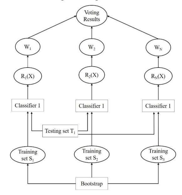
Figure 5 Decision making system.
Table 2 Similarities of the samples.
| Sample | A1 | A2 | A3 | A4 | A5 | A6 | A7 | A8 | A9 | A10 |
|---|---|---|---|---|---|---|---|---|---|---|
| P1 | 1 | 1 | 0 | 0 | 0 | 0 | 0 | 0 | 0 | 0 |
| P2 | 0 | 0 | 0 | 0 | 0 | 0 | 0 | 0 | 1 | 1 |
| P3 | 0 | 0 | 0 | 0 | 1 | 1 | 1 | 1 | 1 | 1 |
D(P1, P2) = 2, D(P2, P3) = 2, and D(P1, P3) = 6 are determined. There are two conclusions:
- 1. P1 and P3 have the same relation to P2, i.e. they have the same distance to P2.
- 2. P1 and P3 are similar to P2; P1 is also similar to P3.
Suppose the abovementioned three examples are instances of malware. Suppose further that these samples contain the value of a variable that is not zero. Table 1 reveals P1 and P2 have no similar characteristics while P2 and P3 have two similar characteristics. That is why the Euclidean distance does not necessarily demonstrate the resemblance of samples in a wide space.
Given the problems described above we followed the SNN approach, which works well in high-dimensional spaces. Jarvis & Patrick [43] first proposed this method. The similarity between two points is featured by the fact that they share a major quarter C with at least k points. This approach has the advantage that it can cluster points of varying densities. As shown in Figure 6, the clustering of varying densities represents circles of different sizes.
In each row of the matrix of similarities the relation of position M between two points is stored. M(A, B) = 1 means that B is nearest to A. In-row saves only k minimum values, and all values are set to 0. The matrix is used to create the nearest K (K-NN) line. From Fig. 10, the points O and P are noise or outliers, but graphs are not used to differentiate them. The extent of the relationship is calculated by:
\[str(0,P) = \sum (k+1-m).(k+1-n)\] (5)
If a point's value is smaller than a unique threshold it looses all edges. In Fig. 10, O and P points are listed as outliers. Ertoz, et al. have focused on the link strength to choose the main points of each cluster with a higher connection capacity. In each cluster, a point is either one of the core points or linked to the core points.
Figure 6 (a) Near neighbor graph and (b) weighted shared near neighbor graph.
The SNN model may be defined as follows:
- 1. calculate the matrix of similarities;
- 2. build the K-NN graph;
- 3. calculate the relation intensity and set the threshold to find low-strength noise and outliers.
- 4. select the high-strength core points;
- 5. assign, or mark as an outlier, a new point to the clustering.
5 Result and Analysis
In the analysis of the research methodology presented in the current work a dataset with 1,40,000 different samples was considered, from which 60% of the data were considered for the purpose of training and the remaining 40% were considered for the testing process. The complete dataset is a collection of benign and malicious files with 70,140 benign files and 69,860 malicious files. Different known classifiers, i.e. Decision Tree, K-Nearest Neighbor, Naïve Bayes, Support Vector Machine, Random Forest, and J48 Decision Tree, were used in the decision making process. The performance of all of the classifiers was evaluated based on the accuracy of the process, which is the percentage of correctly identified instances.
\[Accuracy = \frac{Count (Correctly identified samples)}{Count (Total samples)}\] (6)
5.1 K-Nearest Neighbor
Figure 7 below shows the outcome of the K-Nearest Neighbor method, as can seen in Table 3. The results are shown in terms of the accuracy of each class of malware. Here, the maximum accuracy was 100%, achieved by CyberGate, and the minimum accuracy was 79.2%, achieved by CTB- Locker.
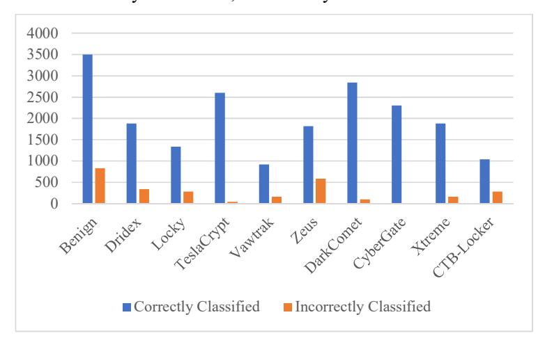
Figure 7 Classification of different classes of malware using k-Nearest Neighbor.
Table 3 shows the classification of files as goodware or malware using K-Nearest Neighbor. As the results show, around 82.3% accuracy was seen for benign files and around 98% accuracy for the malware considered in the dataset. Table 4 below shows the exact accuracy for the classification/ identification of benign
files and malware detected, where the accuracy of the classification of malicious files was about 98%.
Table 3 Detection evaluation using K-Nearest Neighbor.
| S.N. | Family of Sample | Correctly Classified | Incorrectly Classified | Accuracy |
|---|---|---|---|---|
| 1. | Benign | 3499 | 834 | 82.3% |
| 2. | Dridex | 1880 | 340 | 84.2% |
| 3. | Locky | 1340 | 280 | 83.4% |
| 4. | TeslaCrypt | 2600 | 40 | 98% |
| 5. | Vawtrak | 920 | 160 | 84.5% |
| 6. | Zeus | 1820 | 580 | 78% |
| 7. | DarkComet | 2840 | 100 | 96% |
| 8. | CyberGate | 2300 | 0 | 100% |
| 9. | Xtreme | 1880 | 160 | 93% |
| 10. | CTB-Locker | 1040 | 280 | 79.2% |
Table 4 Benign and malicious file accuracy using K-Nearest Neighbor.
| Class | Correctly Classified | Incorrectly Classified | Accuracy |
|---|---|---|---|
| Benign | 3499 | 834 | 82.3% |
| Malicious | 16620 | 1940 | 98% |
5.2 Support Vector Machine
Support Vector Machine was the next algorithm that was tested. In Table 5 and Figure 8, the outcome of the predictions can be seen. The overall accuracy obtained for multi-class classification was 87.6% and for binary classification 94.6%. The maximum accuracy was 100%, achieved by CTB-Locker, and the minimum accuracy was 59.3%, achieved by Vawtrak. Table 6 shows the classification of files as goodware or malware using Support Vector Machine. As the results show, around 83.8% accuracy was seen for benign files and around 89.3% accuracy in the case of malware.
Table 5 Detection evaluation using Support Vector Machine.
| S.N. | Family of Sample | Correctly Classified | Incorrectly Classified | Accuracy |
|---|---|---|---|---|
| 1. | Benign | 3996 | 335 | 93% |
| 2. | Dridex | 1940 | 280 | 87.3% |
| 3. | Locky | 1280 | 340 | 78.7% |
| 4. | TeslaCrypt | 2240 | 400 | 85.1% |
| 5. | Vawtrak | 620 | 460 | 59.3% |
| 6. | Zeus | 1880 | 520 | 79.1% |
| 7. | DarkComet | 2900 | 40 | 98.2% |
| 8. | CyberGate | 2240 | 40 | 98% |
| 9. | Xtreme | 1880 | 160 | 92.1% |
| 10. | CTB-Locker | 1320 | 0 | 100% |
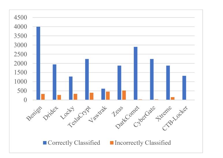
Figure 8 Classification of the different classes of malware using Support Vector Machine.
Table 6 Accuracy of benign and malicious files using Support Vector Machine.
| Class | Correctly Classified | Incorrectly Classified | Accuracy |
|---|---|---|---|
| Benign | 3996 | 8335 | 83.8% |
| Malicious | 16300 | 2240 | 89.37% |
5.3 J48 Decision Tree
J48 Decision Tree was the third algorithm studied (Table 7 and Figure 9). The benefit of the decision tree method is that it works in a 'white box' approach and we can see which decisions resulted from our prediction. Here, maximum accuracy was 100% (Drdex, TeslaCrypt and CyberGateis) and the minimum accuracy was 83.7% (Zeus).
Table 7 Detection evaluation using J48 Decision Tree.
| S.N. | Family of Sample | Correctly Classified | Incorrectly Classified | Accuracy |
|---|---|---|---|---|
| 1. | Benign | 3854 | 477 | 89.7% |
| 2. | Dridex | 2240 | 0 | 100% |
| 3. | Locky | 1460 | 160 | 90.1% |
| 4. | TeslaCrypt | 2240 | 0 | 100% |
| 5. | Vawtrak | 980 | 100 | 91.3% |
| 6. | Zeus | 2000 | 400 | 83.7% |
| 7. | DarkComet | 2840 | 100 | 96.3% |
| 8. | CyberGate | 2240 | 0 | 100% |
| 9. | Xtreme | 1940 | 100 | 95.6% |
| 10. | CTB-Locker | 1280 | 40 | 96.3% |
Table 8 shows the classification of files as goodware or malware using J48 decision tree. As the results show, around 83.8% accuracy was seen for benign files and around 99.5% accuracy in the case of malware.
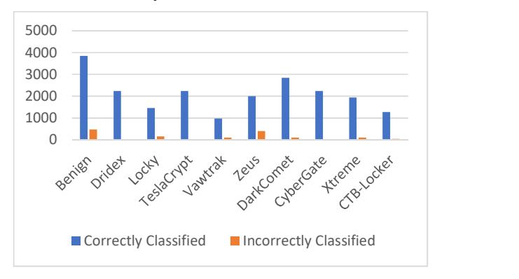
Figure 9 Classification of the different classes of malware using J48 Decision Tree.
Table 8 Accuracy of benign and malicious files using J48 Decision Tree.
| Class | Correctly Classified | Incorrectly Classified | Accuracy |
|---|---|---|---|
| Benign | 3996 | 8335 | 83.8% |
| Malicious | 16300 | 2240 | 99.5% |
5.4 Naïve Bayes
Naïve Bayes was the next algorithm that was evaluated. Table 9 lists the results of the predictions. Here, the maximum accuracy was 100%, achieved by Dark Comet and CTB-Locker, and the minimum accuracy was of 3.5%, achieved by Dridex (Figure 10).
Table 9 Detection evaluation using Naïve Bayes.
| S.N. | Family of Sample | Correctly Classified | Incorrectly Classified | Accuracy |
|---|---|---|---|---|
| 1. | Benign | 2434 | 1897 | 60% |
| 2. | Dridex | 80 | 2140 | 3.5% |
| 3. | Locky | 1520 | 100 | 93% |
| 4. | TeslaCrypt | 2000 | 640 | 93.6% |
| 5. | Vawtrak | 500 | 580 | 50% |
| 6. | Zeus | 1700 | 700 | 72% |
| 7. | DarkComet | 2940 | 0 | 100% |
| 8. | CyberGate | 2240 | 40 | 98.1% |
| 9. | Xtreme | 1880 | 160 | 92.8% |
| 10. | CTB-Locker | 1320 | 0 | 100% |
Table 10 the classification of files as goodware or malware using J48 Decision Ttree. As the results show, around 100% accuracy was seen for benign files and around 68.3% accuracy in the case of malware in the dataset.
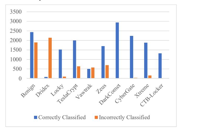
Figure 10 Classification of the different classes of malwares using naïve Bayes.
Table 10 Accuracy of benign and malicious files using naïve Bayes.
| Class | Correctly Classified | Incorrectly Classified | Accuracy |
|---|---|---|---|
| Benign | 4331 | 0 | 100% |
| Malicious | 13180 | 4360 | 68.3% |
5.5 Random Forest
Random Forest was the last algorithm that was tested. The algorithm resulted in good prediction accuracy. Table 4 presents the results of its predictions. Here, the maximum accuracy was 100%, achieved by DarkComet, CyberGate, Xtreme, and CTB- Locker (Figure 11).
Table 11 Detection evaluation using Random Forest.
| S.N. | Family of Sample | Correctly Classified | Incorrectly Classified | Accuracy |
|---|---|---|---|---|
| 1. | Benign | 4138 | 193 | 96.1% |
| 2. | Dridex | 2120 | 100 | 95.7% |
| 3. | Locky | 1520 | 100 | 93.3% |
| 4. | TeslaCrypt | 2640 | 0 | 100% |
| 5. | Vawtrak | 920 | 160 | 84.7% |
| 6. | Zeus | 2120 | 280 | 88.7% |
| 7. | DarkComet | 2940 | 0 | 100% |
| 8. | CyberGate | 2280 | 0 | 100% |
| 9. | Xtreme | 2040 | 0 | 100% |
| 10. | CTB-Locker | 1320 | 0 | 100% |
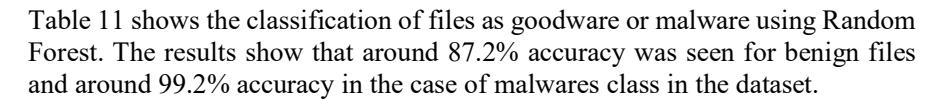
Figure 11 Classification of the different classes of malware using Random Forest.
Table 12 Accuracy of benign and malicious files using Random Forest.
| Class | Correctly Classified | Incorrectly Classified | Accuracy |
|---|---|---|---|
| Benign | 4138 | 193 | 87.2% |
| Malicious | 16580 | 640 | 99.2% |
Figure 12 shows that the different models provided different results in classification. Naive Bayes had the lowest accuracy (100% and 68.3%), followed by K-Nearest Neighbor and Support Vector Machine (82.3%, 98% and 83.8%, 89.37% respectively). The highest precision was achieved with J48 and Random Forest (83.8%, 99.5%, and 87.2%, 99.5% respectively).
Figure 12 Comparison graph for the accuracy of the different classifiers.
6 Conclusion
Because of the ever growing number of malware variants and the variety of malware activities there is renewed interest in and need for effective malware detectors to protect against zero-day attacks. Anti-virus firms typically collect millions of malicious samples, which are obtained and analyzed in the usual manner, delaying the identification of any unusual samples that harm users. Our primary aim was to create a machine-learning system that commonly detects as many malware samples as possible, with the tough constraint of having a zero false positive rate. We came quite close to our goal, but still have a non-zero false positive rate. For this method to become part of a highly competitive commercial product, a number of deterministic exemption mechanisms must be added. In the proposed work, the Random Forest and Naïve Bayes classifiers showed the best results.
The system was validated using a sample of 140,000 files consisting of malware and benign files. The malware was further divided into 9 different classes on the basis of their properties. The complete sample list was categorized into groups at a 60% and 40% ratio for further processing of system training and decision making as training dataset and testing dataset respectively. Given that most antivirus products achieve a detection rate of more than 90% there was a very significant increase in the overall detection rate of 3 to 4% produced by our algorithms.
7 Future Scope
In the future more features will be considered to develop a better model that will use a more robust deep learning technique for the detection of cyber attacks. It will also be capable of detecting all types of different malware attacks and automatically deal with all types of cyber attacks.