
1 Introduction
Security systems must continually be improved to cope with evolving demand. An example of a current challenge is the proliferation of sexual harassment cases against women in public places such as toilets and public transportation. Preventive measures are taken, for example in the form of clearly designated toilets for each gender. Another preventive measure is the use of buses or special train carriages for women. Despite all these attempts, sexual harassment cases still occur. This shows that the currently implemented monitoring and security systems are inadequate. According to the Tokyo Police Department there were 1,750 reports of sexual harassment on public transportation, of which more than 50% occurred on trains [1]. Meanwhile in Indonesia a survey was conducted by the Safe Public Space Coalition (KRPA) involving 62,000 female respondents. This survey showed that 35.45% of female passengers experienced sexual harassment on buses, 30% on city transportation, and 17.79% on KRL trains [2]. These data show that a more sophisticated security system is needed to automatically recognize the gender of people that are trying to access public
facilities designated specifically for women. Such security systems can be implemented based on image processing using face biometric data. The use of biometric data is preferable because it is relatively fast and unintrusive.
Gender recognition based on face biometric data is possible because the facial characteristics of males and females are different. Key information about the gender of a face is conveyed by some broad (though not mutually exclusive) classes of information: (i) superficial and/or local features (such as facial hair, skin texture, width of the mouth, thickness of eyebrows), (ii) configural relationships between features (predominantly defined by ratio between two local features), and (iii) the 3D structure of the face [3].
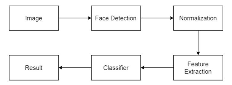
Figure 1 Block diagram of the proposed system.
In this paper, we propose a security system with gender recognition, as shown in Figure 1. First, face detection is performed on the input image using the Viola-Jones method. Then in the normalization step the face is cropped from the input image and resized to a standard size. After that, feature extraction is carried out to extract features from the face images that will be used in classification. Finally, in the classification step, a classifier uses the extracted features to classify the face images according to their class, namely female or male.
The images that we used in this study were obtained from the VISiO Lab and CASIA datasets. In a previous work [4], the authors also used the VISiO Lab face dataset for a gender recognition system using principal component analysis (PCA) and linear discriminant analysis (LDA). The authors reported an accuracy rate of up to 82.90% and 85.90% for PCA and LDA classifiers, respectively. One main limitation of this work is the need to perform manual cropping of the facial areas. With the system proposed in this paper we aim to improve the overall accuracy of the system and also implement automatic cropping of the facial area. A second dataset used in the current study is the CASIA dataset. This dataset was developed for use in anti-face-spoofing research [5]. To the best of the authors' knowledge, this dataset has never been used before in automatic gender recognition research. Therefore, there is currently no automatic gender
recognition system that has been tested using this dataset with which to compare the performance of the system we propose in this paper.
In [5] the authors used Quaternionic Local Ranking Binary Pattern (QLRBP) as feature extractor to prevent face-spoofing, i.e. the use of pictures/videos of a legitimate user by an attacker to gain access to an asset protected by a facial biometric security system. The authors showed that the use of QLRBP gave satisfactory results, yielding an accuracy rate of up to 95.20% using kNN and an accuracy rate of 97.36% using SVM. These results show that QLRBP can extract facial features and is therefore a good candidate for a feature extractor in a gender recognition system. An example of the use of Multi Level Local Phase Quantization (MLLPQ) is provided by [6], in which gender and age recognition were performed based on facial data. The experiments showed that an accuracy rate of 79% could be achieved. Another example is provided by [7], in which the authors used MLLPQ to determine kinship based on facial data. The authors reported an accuracy level of 82.86% using MLLPQ.
In this paper, we propose and compare the performance of a gender recognition system based on the combination of two different feature extractors, namely QLRBP and MLLPQ, and two different classifiers, namely kNN and SVM. The performance was evaluated on two aspects, namely the accuracy and the speed of the system.
The rest of this paper is organized as follows: in Section 2 we discuss the proposed system in more detail, in Section 3 we present the results of our experiments and finally in Section 4 we present our conclusions and pointers for future work.
2 Material and Method
2.1 The Dataset
We used the Multiview face database of the Video, Image and Signal Processing (VISiO) laboratory Satya Wacana Christian University (SWCU). This database currently contains face images of 100 subjects, equally distributed according to gender (i.e. 50 subjects are female and 50 subjects are male) with age varying between 19 and 69 years. The images were taken under controlled conditions in our laboratory. Each subject was photographed against a uniform white background using a single camera and identical settings [8].
Then we added the CASIA Face Image Database, Version 5.0 (or CASIA-FaceV5), which is the latest updated CASIA dataset for faces and consists of a total of 2,500 colored facial images of 500 different subjects (persons). The images of faces in this dataset were captured in a single session using a specific Logitech USB camera. The subjects in this dataset are not professional research scholars but they are normal people like graduate students, workers, waiters, etc. [9].
2.2 Feature Extractor & Classifier
Feature extraction can be done with several techniques, such as Gabor Features, Local Binary Pattern (LBP), Local Phase Quantization (LPQ), Scale – invariant Feature Transform (SIFT), Histograms of Oriented Gradients (HOG), etc. [10]. There are some feature extractors that have been developed from existing ones, such as Quarternionic Local Ranking Binary Patterns (QLRBP), which was developed from Local Binary Patterns (LBP) [11], and Multi Level Local Phase Quantization (MLLPQ) which was based on Local Phase Quantization (LPQ) [12]. The functionality of LPQ is similar to that of LBP [13], but LBP operates in the spatial domain, whereas LPQ operates in the frequency domain.
We used a classifier to separate the output data obtained by feature extraction into classes. Examples of classifier methods are [14] Decision Tree (DT), Support Vector Machine (SVM), Artificial Neural Network (ANN), k-Nearest Neighbor (kNN), etc. The classifier needs the correct choice of parameters to produce high quality classification [15]. For example, the SVM classifier uses the kernel function parameter to solve nonlinear multi classification problems [16]. Meanwhile, the kNN classifier uses the k parameter (number of nearest neighbors) to determine the class, following the majority [17].
One of the simplest classifiers to implement is the kNN [18]. Even though this classifier is simple it also has some other advantages [19]: it is relatively easy to learn, the training process is very fast, it is resistant to noisy training data and effective when the training data set is large. Another classifier option is SVM. This classifier is more complicated to implement compared to kNN, but it has the following advantages [20]: it can solve classification and regression problems linearly as well as non-linearly and is able to solve dimensionality problems [21]. SVM also has high accuracy and a relatively small error value as well as the ability to overcome overfitting [22].
2.3 Quarternionic Local Ranking Binary Pattern (QLRBP)
Quarternion numbers are four-dimensional complex numbers consisting of one real component and three imaginary components. The general form of the quarternion number is in Eq. (1) as follows:
\[\dot{q} = a + ib + jc + kd \tag{1}\] where a, b, c, and d are real numbers while i, j, and k are complex operators. In image processing applications, the imaginary part of the quarternion is used to represent color pixels according to the following mapping: in Eq. (2)
\[\dot{q} = ir + jg + kb \tag{2}\] where r, g, and b are the red, green, and blue components, respectively.
Quarternionic Local Ranking Binary Pattern (QLRBP) [11] extracts features in the quarternionic domain directly. The obtained quarternion representation is transformed using Clifford Translation of Quarternion (CTQ). The resulting phase of the CTQ transformation is then converted into a QLRBP image by means of Local Binary Pattern (LBP). The histogram of the QLRBP image is taken as the feature vector of the input image.
2.4 Multi Level Local Phase Quantization (MLLPQ)
The Local Phase Quantization (LPQ) method is based on the quantized phase of the discrete Fourier transform (DFT) computed in local image windows [23]. LPQ is also based on the blur invariance property of the Fourier phase spectrum [6]. The local phase information is extracted using 2D DFT or the short-term Fourier transform computed over a rectangular \(M \times M\) neighborhood \(N_x\) at each pixel position x of the image f(x), defined by Eq. (3) [6]:
\[F(u,x) = \sum_{y \in N_{x}} f(x-y)e^{-j2\pi u^{T}y} = w_{u}^{T} f_{x}\] (3)
where \(w_u\) is a basis vector of the 2D Discrete Fourier Transforms at frequency \(\boldsymbol{u}\) and \(\boldsymbol{f_x}\) is another vector that contains all \(M^2\) image samples of \(N_x\) [23].
In [13], a face image is processed using the Local Binary Patterns algorithm and then divided into 3 × 4 sub-blocks. This method is called Multi Block Local Binary Patterns (MBLBP), which gives better results because it provides more specific information/data. Inspired by MBLBP, the authors proposed MBLPQ in [6]. In order to outperform MBLPQ, Multi Level Local Phase Quantization (MLLPQ) was employed to obtain more relevant data [6].
The main idea of MLLPQ is to extract features from various MBLPQ divisions and then combine them. It is done by extracting the features of the whole image, then dividing the image into \(2^2\) sub-blocks and extracting the features of each sub-block, and so on until it meets the desired level. The final result of the MLLPQ are \(1^2 + 2^2 + .... + n^2\) histograms. Finally, the feature vector can be acquired by combining these histograms. Figure 2 shows an example of MLLPQ with 3 levels.
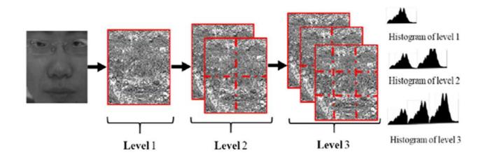
Figure 2 Example of feature extraction using MLLPQ with 3 levels [13].
2.5 Proposed Methods
2.5.1 Data Collection
The datasets used in this study were obtained from VISiO Lab [24] and CASIA FaceImageDatabase Version5.0 (or CASIA-FaceV5) [25], as shown in Figure 3. A total of 700 images, consisting of 350 male and 350 female images, were randomly selected from the two datasets.
Figure 3 (a) The VISiO Lab image; (b) the CASIA-FaceV5.
This study used frontal pose images of both males and females with several variations as training data. The variations include the physical traits (length of hair, skin color, etc.) and accessories worn by the models (glasses, teeth braces, etc.).
2.5.2 Data Processing
The facial image data are pre-processed prior to the classification stage. Facial image size normalization is done to provide images of equal size, i.e. 80 × 80 pixels. This is done so that the feature vectors are not too large, which might lead to excessive processing load.
Then, the features of the image are extracted using QLRBP and MLLPQ. The QLRBP method yield three histograms of each color channel (R, G, and B) and these three histogram vectors are combined into a single vector. In order to acquire more detailed data, the resulting image is divided into blocks of various sizes, starting from 1 × 1 (consisting of 1 block) to n × n (consisting of n 2 blocks).
Each block is represented by one feature vector. The vector(s) are then used in the classification process. Meanwhile, the MLLPQ method carried out feature extraction by using only the pixel luminance values. Like the QLRBP method, the MLLPQ method also divides the image into blocks of various sizes, starting from \(1 \times 1\) (consisting of 1 block) to \(n \times n\) (consisting of \(n^2\) blocks). Finally, the feature vector is obtained by combining all of the histogram vectors. Figure 4 shows an example of image division into blocks.
Figure 4 (a) \(1 \times 1\) block, (b) \(2 \times 2\) block, (c) \(3 \times 3\) block, (d) \(4 \times 4\) block.
2.3.3 Performance Evaluations
The proposed system was evaluated mainly based on the accuracy rate it could achieve. The accuracy was calculated by Eq. (4):
\[Accuracy = \frac{The \ correct \ amount \ of \ data}{Total \ data} \times 100\%\] (4)
Meanwhile, the error was formulated by Eq. (5):
\[Error = 100\% - Accuracy \tag{5}\]
Additionally, we also considered the processing speed of the algorithms when evaluating the performance of the system.
3 Results and Discussion
To simulate the proposed study, we used the MATLAB R2017a software and a laptop with an AMD Ryzen 7 3700U processor and 8 GB of RAM.
3.1 Feature Extraction using QLRBP
The QLRBP method requires a normalized image in RGB format for extracting the features, as depicted in Figure 5. The length of the feature vector and the processing time are subject to the number of blocks used, as shown in Table 1.
Figure 5 (a) Input image, (b) result of QLRBP in the R domain, (c) result of QLRBP in the G domain, (d) result of QLRBP in the B domain.
3.2 Feature Extraction using MLLPQ
The MLLPQ method requires a normalized image in greyscale format. The length of the feature vector and the processing time are subject to the number of blocks used, as shown in Table 1. Images that have previously been normalized cannot be used directly by this method, because the MLLPQ method only uses the pixel luminance data from the image. Therefore, the image must first be converted to a greyscale image, as depicted in Figure 6.
Table 1 Result of feature extraction.
| Number of Blocks | QLR | BP | MLLPQ | ||
|---|---|---|---|---|---|
| Length of the Feature Vector | Processing Time (ms) | Length of the Feature Vector | Processing Time (ms) | ||
| 1 | 768 | 389.0 | 256 | 20.0 | |
| 4 | 3,072 | 438.0 | 1,280 | 36.0 | |
| 9 | 6,912 | 511.3 | 3,584 | 72.8 | |
| 16 | 12,288 | 619.4 | 7,680 | 132.4 | |
| 25 | 19,200 | 764.0 | 14,080 | 227.7 | |
| 36 | 27,648 | 933.0 | 23,296 | 360.6 | |
Figure 6 (a) Input image, (b) greyscale image, (c) result of feature extraction.
3.3 Accuracy
The basic difference between QLRBP and MLLPQ is the length of the feature vector. QLRBP gives a longer feature vector since it employs the R, G, and B color components of the input image, whereas MLLPQ utilizes only the pixel luminance values. The kNN classifier uses the Num Neighbors parameter, which defines the number of neighbors. Meanwhile, the SVM classifier uses the kernel function parameter, which includes linear, RBF, and polynomial functions. By default, the SVM classifier uses the linear kernel function because of its simplicity. However, for RBF and polynomial kernel functions, additional parameters are necessary to achieve optimum results as they are non-linear classifiers.
It is necessary to adjust the kernel scale parameter when applying the RBF kernel function [26]. The value of the kernel scale parameter is within the range of 0.001 to 1000 [27]. In this study, the option 'auto' was chosen to determine the kernel scale parameter. The values of the kernel scale parameter for QLRBP and MLLPQ are given in Tables 2 and 3, respectively. Meanwhile, the polynomial order parameter must be assigned to an integer number when applying the polynomial kernel function [21]. In this study, the polynomial order was set to 1 because it gave the best results based on our experiments, as shown in Table 4.
A performance comparison of all methods is presented in Table 5. The testing was conducted by means of 5-fold cross validation to optimize the accuracy rate and processing time. The results presented in Table 5 are the averages of the results obtained for all numbers of blocks. The largest number of blocks had the highest accuracy because this contains the most detailed information of the image. However, a larger number of blocks also means that the total length of the feature vectors for the image is much longer. Based on Table 5, the accuracy of the kNN classifier performed better than SVM. The extracted feature vectors using MLLPQ were shorter than those of QRLBP. Yet, MLLPQ outperformed QLRBP in terms of both accuracy and processing time, as can be inferred from Figures 7-8.
For the kNN classifier, the value k was inversely proportional to the accuracy. This suggests that the boundary between the two classes cannot easily be identified. In other words, it suggests that data from one class form small clusters (or 'islands') that are surrounded by data from the other class. Therefore, when the classifier considers more than 2 neighbors, in many cases they will end up misclassifying the data. Meanwhile, the results given by the SVM classifier using different kernel functions and different parameters, were approximately identical. From Table 5 it can be inferred that the MLLPQ method paired with the kNN classifier with k = 1 gave the highest accuracy at 92.11%.
Although this system has higher accuracy compared to previously published works ([4] and [6]), these results were obtained in a controlled environment. The proposed system is yet to be tested in a real-life setting. Also, while the accuracy obtained is quite satisfactory, there is still room for improvement to increase the accuracy even further. Furthermore, the system as implemented in this study is unsuitable for real-time application because the highest speed achieved in our experiments was only around 22.22 fps.
Table 2 Scale values of SVM classifier using RBF kernel function for QLRBP.
| Number | Iteration | |||||
|---|---|---|---|---|---|---|
| of Blocks | st 1 | 2nd | 3rd | 4th | 5th | |
| 1 | 30.11 | 30.04 | 30.03 | 29.84 | 30.15 | |
| 4 | 68.89 | 68.02 | 68.25 | 68.37 | 68,43 | |
| 9 | 106.64 | 105.96 | 107.23 | 106.2 | 106.46 | |
| 16 | 144.71 | 146.98 | 144.26 | 143.77 | 145.15 | |
| 25 | 182.88 | 183.79 | 181.82 | 180.29 | 183.08 | |
| 36 | 216.03 | 218.35 | 218.81 | 218.29 | 217.20 | |
Table 3 Scale values of SVM classifier using RBF kernel function for MLLPQ.
| Number | Iteration | ||||
|---|---|---|---|---|---|
| of Blocks | st 1 | 2nd | 3rd | 4th | 5th |
| 1 | 17.62 | 17.24 | 17.44 | 17.34 | 17.41 |
| 4 | 43.50 | 43.09 | 43.08 | 43.48 | 43.32 |
| 9 | 75.79 | 75.48 | 75.70 | 75.60 | 75.67 |
| 16 | 112.98 | 113.20 | 113.09 | 113.67 | 113.21 |
| 25 | 155.18 | 155.77 | 156.34 | 155.56 | 155.27 |
| 36 | 202.28 | 201.76 | 201.44 | 201.41 | 202.17 |
Table 4 Accuracy obtained using various polynomial orders.
| Number | Accuracy (%) | ||||||
|---|---|---|---|---|---|---|---|
| of Blocks | QLRBP | MLLPQ | |||||
| Order 1 | Order 2 | Order 3 | Order 1 | Order 2 | Order 3 | ||
| 1 | 75.71 | 73.26 | 50.00 | 82.57 | 78.14 | 70.14 | |
| 4 | 81.86 | 76.29 | 66.29 | 88.86 | 86.14 | 61.57 | |
| 9 | 85.57 | 63.57 | 60.71 | 91.57 | 87.86 | 67.57 | |
| 16 | 90.00 | 51.14 | 69.71 | 92.71 | 86.43 | 56.57 | |
| 25 | 91.00 | 65.57 | 69.86 | 93.71 | 54.86 | 67.57 | |
| 36 | 89.57 | 61.14 | 56.57 | 94.86 | 62.43 | 72.14 | |
| Cla | Classifier | Error (%) | Time (s) | |||||
|---|---|---|---|---|---|---|---|---|
| QLRBP | ||||||||
| k = 1 | 89.95 | 10.05 | 42.4 | |||||
| k = 3 | 88.78 | 11.22 | 42.21 | |||||
| kNN | k = 5 | 87.20 | 12.80 | 42.60 | ||||
| k = 7 | 86.59 | 13.41 | 42.20 | |||||
| k = 9 | 86.06 | 13.94 | 42.17 | |||||
| Linear | 85.64 | 14.36 | 150.57 | |||||
| SVM | RBF | 84.27 | 15.73 | 164.91 | ||||
| Polynomial | 85.83 | 14.17 | 141.01 | |||||
| MLLPQ | ||||||||
| k = 1 | 92.11 | 7.89 | 32.18 | |||||
| k = 3 | 89.02 | 10.98 | 31.87 | |||||
| kNN | k = 5 | 87.72 | 12.28 | 31.82 | ||||
| k = 7 | 87.18 | 12.82 | 32.15 | |||||
| k = 9 | 86.67 | 13.33 | 33.63 | |||||
| Linear | 90.14 | 9.86 | 90.61 | |||||
| SVM | RBF | 90.23 | 9.77 | 103.92 | ||||
| Polynomial | 90.49 | 9.51 | 91.33 | |||||
Table 5 Performance comparison.
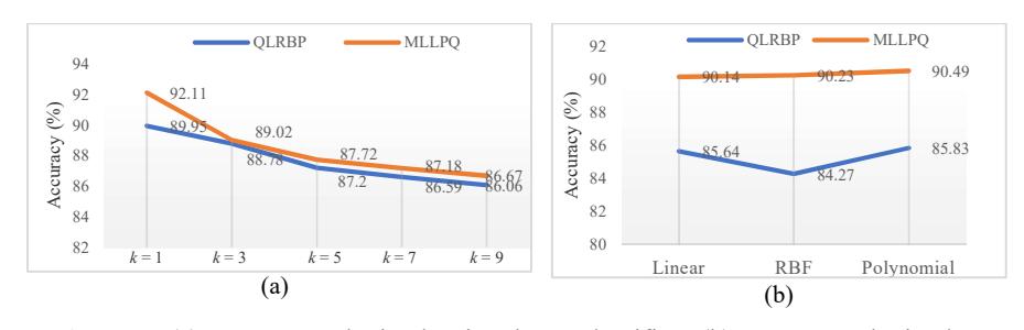
Figure 7 (a) Accuracy obtained using kNN classifier, (b) accuracy obtained using SVM classifier.
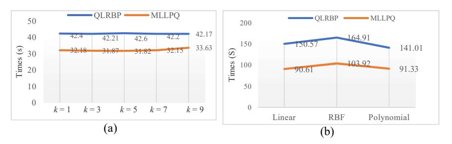
Figure 8 (a) Time elapsed using kNN classifier, (b) time elapsed using SVM classifier.
4 Conclusion
A performance analysis for gender recognition was done using QLRBP and MLLPQ as feature extractors, combined with SVM and kNN as classifiers. The results demonstrated that kNN gave better accuracy than SVM using the kernel parameters as reported in the previous section. Meanwhile, MLLPQ produced shorter feature vectors compared to QLRBP. In addition, MLLPQ was able to yield higher accuracy than QLRBP with both classifiers. In terms of processing time MLLPQ also outperformed MLLPQ with both classifiers. The combination of MLLPQ + kNN was found to be the most accurate method with k = 1, giving an accuracy of 92.11%. In the future, further research will be carried out to optimize the classifiers in order to produce better results. Also, this system should be tested in a real-life environment. Finally, we aim to optimize the system to achieve real-time speed.