
1 Introduction
Much attention has been paid to the utilization of mobile robots in a variety of automated industrial environments. Mobile robots are increasingly used in a wide range of applications that includes many services like planet exploration, surveillance, landmine detection, etc. In all these applications, the locomotion mechanism is an important requirement of the mobile robot to navigate unhindered throughout its environment. The most crucial issue to attain autonomous mobile robots is collision-free path planning. Path planning for mobile robots is concerned with generating a path from a starting point to a goal point, with the provision of optimized performance criteria, including avoiding obstacle collision, reducing the time interval, and decreasing the path traveling
cost. Minimum distance is a very commonly adopted criteria that have to be attained [1,2].
The essential path-planning problem is to create a path for a moving object that satisfies obstacle-collision avoidance. Thus, it is considered as a nondeterministic polynomial time (NP) complete problem. That means the required computational time for solving the path planning problem increases dramatically depending on the problem size increase. So that, it is difficult to apply traditional optimization methods in finding the shortest robot path in real time [3]. Optimization can be defined as the process of searching and determining the best solution or values to given problems according to certain constraints by adjusting the restricted variables to desired characteristics that optimize the objective. The searching process can be achieved using multiple agents that essentially form an evolving agents system. Moreover, the evolving system can be upgraded by iterations depending on a set of mathematical equations or rules. [4]. Swarm intelligence (SI) is an emerging research field of biologically inspired artificial intelligence that discusses the collective behavior within self-organizing societies of agents and decentralized systems. Recently, the implementation of methods of swarm intelligence involving a wide range of applications that demand robustness and flexibility, for example in optimization, robot control, and routing and load balancing in new-generation mobile telecommunication networks.
The various forms of swarm intelligence optimization methods include ant colony optimization (ACO), particle swarm optimization (PSO), artificial bee colony (ABC), and many others [5,6]. However, the firefly algorithm (FA) is one of the most promising swarm-intelligence optimization techniques [7]. FA is a modern swarm intelligence method that can be used for effectively dealing with optimization and NP-hard problems. FA is one of the stochastic algorithms that applies a specific kind of randomization while searching a series of solutions. FA simulates the natural flashing lights of fireflies, which have two fundamental functions: to attract partners or potential prey or to act as a protective warning toward predators [8]. This study aimed to obtain an optimal trajectory for a mobile robot by using a method based on integration of the firefly algorithm and cubic polynomial equations based on the A* algorithm. The objective of the proposed integrated method is to generate the shortest mobile robot path and provide a smooth trajectory that satisfies constraints of motion and moves the robot from a start to goal by avoiding all fixed obstacles.
1.1 Point to Point Trajectories Planning Using Cubic Polynomial Equation
Trajectory planning can be described as a time function that is concerned with determining a potential path. The amount of time during which the trajectory is carried out can be specified as (\(t_f\)-\(t_0\)). The path can be constructed by accepting a set of variables and producing a series of time-based intermediate via points for the mobile robot [9].
The Cubic Polynomial Trajectories technique is one of the essential techniques that generate a smooth trajectory within a specified time. Cubic polynomial trajectory is specified in terms of the position in addition to velocity of the robot in order to generate a smooth curve. Thus, it has four constraints, which are as initial and final positions for each one of the configurations and velocities [9].
\[q(t) = a_0 + a_1 t + a_2 t^2 + a_3 t^3\] (1)
According to Eq. (1), at a time \(t_0\), the initial position and velocity equations are:
\[q(t_0) = q_s \tag{2}\]
\[\dot{q}(t_0) = v_s \tag{3}\]
\((q_s \text{ and } v_s)\) represent the initial position and velocity, respectively. Meanwhile, at time \(t_f\), the final position and velocity equations are:
\[q(t_f) = q_g \tag{4}\]
\[\dot{q}(t_f) = v_q \tag{5}\]
In Eqs. (4) and (5), \((q_g \text{ and } v_g)\) represent the target position and velocity, respectively. Depending on an appropriate number of derivatives for Eq. (1), the following equations have been obtained:
\[q_0 = a_0 + a_1 t_0 + a_2 t_0^2 + a_3 t_0^3 \tag{6}\]
\[v_0 = a_1 + 2a_2t_0 + 3a_3t_0^2 \tag{7}\]
\[q_f = a_0 + a_1 t_f + a_2 t_f^2 + a_3 t_f^3 \tag{8}\]
\[v_f = a_1 + 2a_2t_f + 3a_3t_f^2 (9)\]
In the formulated equation above, the parameters that should be computed are the joint angle of each initial, intermediate, and goal point, and the joint angular velocity of each initial, intermediate, and goal point. The result of implementing the cubic polynomial equations is a smooth trajectory that starts from the initial point, passes through intermediate points, and terminates at the goal point [9,10].
2 Firefly Algorithm
The firefly algorithm (FA) belongs to the category of swarm intelligence-based algorithms. The FA algorithm operates on the principle that simulates the social behavior and the communications mechanism of firefly via luminescent flashes.
The main usage of these flashes is to attract a mating partner or for protection against predators. However, the two essential issues in the FA algorithm involve the light intensity variation and attractiveness formulation [11, 12].
The firefly algorithm mainly depends on the physical formula for light intensity I, which decreases automatically with the increase of distance \(r^2\), where \(I \propto r^2\). In contrast, the light absorption by the air increases dramatically with increasing distance from the source. Therefore, the light intensity is specified to be proportionate to the fitness function of the problem to be solved [11,12]. The formulation of the firefly algorithm is based on the idealization of the flashing characteristics of fireflies, involving:
- 1. The entire fireflies are unisex. Therefore, one firefly will be attracted to other fireflies without paying attention to their sex.
- 2. The attractiveness of a firefly is proportional to their brightness, which decreases when their distance increases. However, if there are two different flashing fireflies, a less bright firefly will be attracted by and move towards a brighter one. When there is no brighter firefly, the firefly will move randomly.
- 3. Firefly brightness is determined by an objective function [13].
FA is a population-based algorithm. The population members represent individual fireflies that are flying through the search space and each firefly is considered a candidate optimal solution for the problem to be solved. The candidate problem solution si is represented as:
\[s_i = (s_{i1}, ..., s_{iD}) \quad for \ i = 1, ..., N\] (10)
where N demonstrate the size of the population and D demonstrate the dimensionality of the problem. For each solution s in the standard firefly algorithm, the firefly's light intensity I is proportional to the value of the corresponding fitness function, and the light absorption is approximated using the fixed light absorption coefficient \(\gamma\). Moreover, the light intensity I(r) is adjusted depending on the light absorption coefficient according to the following equation:
\[I(r) = I_0 e^{-\gamma r^2} \tag{11}\] where \(I_0\) represents the light intensity of the source. The fireflies' attractiveness \(\beta\) is proportional to their light intensity I(r). Moreover, the attractiveness \(\beta\) is adjusted according to the following equation:
\[\beta = \beta_0 e^{-\gamma r^2} \tag{12}\] where \(\beta_0\) demonstrate the attractiveness at distance r = 0. The distance between any two fireflies \(x_i\) and \(x_j\) is expressed as the Euclidean distance by the base firefly algorithm, as follows:
\[r_{ij} = \|\mathbf{s}_i - \mathbf{s}_j\| = \sqrt{\sum_{k=1}^{k=N} (\mathbf{s}_{ik} - \mathbf{s}_{jk})^2}\] (13)
Dependently, the movement of the i - th firefly is attracted to another more attractive firefly j. In this manner, the following equation is applied:
\[\mathbf{s}_i = \mathbf{s}_i + \beta_0 e^{-\gamma r^2} + \alpha \varepsilon_i \tag{14}\] where \(\varepsilon_i\) is a random number drawn from a Gaussian distribution. In the firefly algorithm, the fireflies' movements comprise three terms: the current position of the i-th firefly, the attraction to another more attractive firefly, and random moving. Moreover, random moving of a firefly is determined by randomization parameter \(\alpha\) and a randomly generated number from the interval [0,1]. However, in the case of firefly attractiveness \(\beta_0 = 0\), the movement relies completely on a random walk. Meanwhile, the light absorption coefficient \(\gamma\) plays a crucial influence on the speed of convergence. Accordingly, the value of the light absorption coefficient can be set from the interval \(\gamma \in (0, \infty)\) based on the problem to be optimized. Typically, it varies from 0.1 to 10.
Pseudo-code of the FA is illustrated in Algorithm 1:
Algorithm 1. Pseudocode of the basic firefly algorithm
Input: Population of fireflies x
=(x_1,...,x_N), objective function f(x_i).
Output: The best solution x_{best} and its value f_{min}
                  = min (f(x_{best})).
1: generate initial population \mathbf{x}^{(0)} = (\mathbf{x}_1^{(0)}, \dots, \mathbf{x}_N^{(0)}).
2: f(x_i^{(0)})
= evaluate new solution and update light intensity.
3: t = 0.
4: while t < MAX\_GEN do
5: for i = 1 to N do
    for j = 1 to N do
6:
7:
       if I_i > I_i then
8:
        move firefly i towards j.
9:
       end i
10: end for
11: f(x_i^{(t)}) = evaluate new solution.
12: update light intensity
13: end for
14: rank fireflies and find the best.
15: t = t + 1
16: end while
The firefly algorithm runs on the following principle: an initial population of fireflies is assigned randomly. The firefly search process is iteratively operated and is composed of the next steps: the initial value of parameter is alternated. Secondly, an evaluation function evaluates the quality of the solution. Thirdly, the population of fireflies is sorted according to their fitness values. Fourthly, the best individual in the population is selected. Finally, a movement function performs a move of the firefly positions in the search space. However, the fireflies are moved towards a more attractive individual. Eventually, the iterative firefly search process is terminated as soon as the maximum number of fitness function evaluations is attained [14-17].
3 A* Algorithm
The A* algorithm is a best-first search algorithm, which is concerned with generating the least cost path from a start point to a goal point. The most significant aspect of the A* algorithm is a good heuristic estimate function, which improves the efficiency and performance of the algorithm. The A* algorithm produces an optimal path to a goal if the heuristic function ℎ() is admissible [14]. It is an extension of the Dijkstra algorithm. The A* algorithm uses the function:
\[F = g(n) + h(n), \tag{15}\] where g(n) is the path-cost function, which denotes the cost from the starting node to the current node; h(n) is the heuristic estimate function of the distance from the current node to the goal node. The A* algorithm is used to solve assumption-based path planning by navigating and exploring an environment to find the minimum cost path from a specific start to goal point.
The A* algorithm begins searching from the starting point. As soon as it moves across the graph, it keeps track of the path segment with minimum cost while maintaining other alternate path segments in a sorted priority queue. At every movement, the A* algorithm repeatedly checks the cost of a segment of the path being traversed. However, in case the cost of the path segment being traversed is higher than another encountered path segment, it abandons the path segment with higher cost and instantly traverses the lower-cost path segment instead. This process is iteratively executed until reaching the goal point [18]. Several studies have used A* in robot solutions [19,20].
3.1 Proposed Firefly Algorithm Method for Mobile Robot Path Planning
Finding the shortest path being considered as the optimization problem that was intended to determine a potentially shortest route from a start point to a goal point.
The integration of the firefly algorithm with cubic polynomial trajectories was used to construct the shortest collision-free smooth path for a mobile robot. The principle of operation of the proposed method is planning the quickest smooth path within a free Cartesian space according to two iterative processes: construction of the free space, followed by the generation of the shortest smooth path.
Importantly, the proposed method completely operates within a free area to provide guaranteed collision-free planning. Initially, the free space in the mobile robot environment is constructed by analyzing the robot environment to find collision points and collision-free points. The collision points are found by intersecting the robot and obstacles areas, where the remaining points are considered free-space points. In the case of obstacles being formulated as circles, the collision checking function is:
\[d_{L1} = \sqrt{(x - x_{c1})^2 + (y - y_{c1})^2}\] (16)
\[d_{L2} = \sqrt{(x - x_{c2})^2 + (y - y_{c2})^2}\] (17)
\[d_{Ln} = \sqrt{(x - x_{cn})^2 + (y - y_{cn})^2}\] (18)
\[v = \max\left(1 - \frac{d_L}{r}, 0\right) \,\forall d_L \in \{d_{L1}, d_{L2}, \dots, d_{Ln}\}\] (18)
where \(d_{L1}\), \(d_{L2}\), \(d_{Ln}\) represent the distances between the robot and the center of a circular obstacle \((x_c, y_c)\). In addition, v represents the verification value of the collision checking function. As soon as the free space has been constructed, the proposed method of A* algorithm and the firefly algorithm starts planning the shortest smooth path within the free space according to two iterative processes: construction of the shortest robot path process followed by the smooth trajectory generation process.
Moreover, the A* algorithm is initialized by placing the start node as the 'current node' in the open list, which is inserted into the currently planned path. Subsequently, the current node is expanded to eight connected neighborhood nodes for determining the next arm movement, i.e. the candidate next nodes. Only nodes that belong to the free Cartesian are used. Accordingly, the cost value is computed for each of these neighborhood nodes by implementing the following heuristic cost function:
\[F = g(n_f) + h(n_f) \qquad \forall n_f \in N^k\] (20)
The parameters \(g(n_f)\) are the path-cost from the starting node to the current node that belongs to the free space and \(h(n_f)\) is the heuristic estimate function of the distance from the current node that belongs to the free space to the goal node.
\(N^k\) contains only the set of neighbor nodes that belong to the free space and have not yet been visited by the current \(A^*\) algorithm movement. After that, the expanded neighborhood nodes with associated cost values are placed in the queue open list in a descending manner. Ultimately, this iterative process of node expansion and selection is terminated as soon as the goal point is appended to the closed list. Consequently, the path generated by implementation of the \(A^*\) algorithm is considered the best shortest path and the cost function is applied to the generated path according to Eq. (24).
While in the process of smooth trajectory generation, the cubic polynomial equations and the firefly algorithm are applied for smooth trajectory generation based on the generated path of the A* algorithm. First, the set of free collision paths for the mobile robot is generated by randomly selecting a specific number of intermediate points to formulate the initial firefly population. However, a specific number of intermediate points are selected randomly from the free space. After that, the cubic polynomial equations are used to generate the corresponding path that connects each subsequence points together.
\[q_x(t) = a_0 + a_1 t + a_2 t^2 + a_3 t^3 (21)\]
\[q_{\nu}(t) = a_0 + a_1 t + a_2 t^2 + a_3 t^3 \tag{22}\]
Accordingly, the initial and final positions at time \(t_0\) and \(t_f\) are:
\[q_{x_0}(t_0) = q_{s_x} (23)\]
\[q_{y_0}(t_0) = q_{s_y} (24)\]
\[q_{x_f}(t_f) = q_{g_x} \tag{25}\]
\[q_{y_f}(t_f) = q_{g_y} \tag{26}\]
Subsequently, the collision checking equation is operated to check for collisions on the generated path. In case there are no collisions between the path points and obstacles, the generated path is accepted. Otherwise, the generated path is ignored, and other collision-free points from the mobile robot environment are randomly selected to generate an alternative path. Then, the Euclidean distance is applied to calculate the fitness function (distance cost) to each acceptable path, according to:
Trajectory cost = \[\sum_{i=1}^{m} \sqrt{(x_i - x_{i+1})^2 + (y_i - y_{i+1})^2}\] (27)
Moreover, the set of acceptable paths represents a candidate solution of the mobile robot path planning problem and is formulated as an initial firefly population, as demonstrated in Figure 1. Parameter D denotes the number of selected intermediate points. Subsequently, the specific number of firefly algorithm iterations is iteratively operated to update the light intensity and the attractiveness for each path.
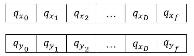
Figure 1 Vector of selected intermediate points.
The i-th firefly is attracted to another, more attractive firefly j, and the movement equation is applied for each x and y coordinate of the intermediate via points as follows:
\[\mathbf{s}_{xi} = \mathbf{s}_{xi} + \beta_0 e^{-\gamma r^2} + \alpha \varepsilon_i \tag{28}\]
\[\mathbf{s}_{vi} = \mathbf{s}_{vi} + \beta_0 e^{-\gamma r^2} + \alpha \varepsilon_i \tag{29}\]
Depending on the modified movement of the i-th firefly, the cubic polynomial equations are applied to generate the corresponding path that connects each subsequent intermediate via point together. After that, the collision checking equation is operated to check for collisions on the currently generated path. In case there are no collisions between the path points and obstacles, the generator path is accepted and added to the updated population. Otherwise, the generated path is ignored.
Based on the updated population of the firefly algorithm, the firefly algorithm iteratively updates the light intensity, attractiveness, and movement of each path for a specific number of iterations. Finally, the best path from whole firefly algorithm iterations with minimum cost function is considered a free-collision shortest path for the mobile robot. Figure 2 shows a flowchart of the proposed method.
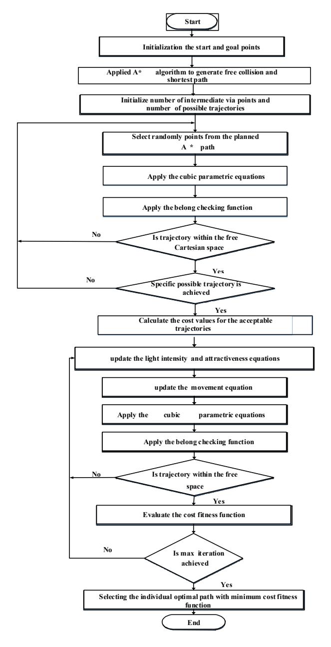
\(\begin{tabular}{ll} Figure 2 & The proposed method of firefly algorithm for mobile robot path planning. \end{tabular}\)
Pseudo-code of the proposed FA method is shown in Algorithm 2:
Algorithm 2. Pseudo code of the proposed FA method
Input: Population of fireflies x = (x_1, ..., x_N), objective function f(x_i)
Output: The best solution x_{best} and its value f_{min} = min(f(x_{best}))
1: apply A * algorithm, and generate initial population
\mathbf{x}^{(0)} = (\mathbf{x}_1^{(0)}, \dots, \mathbf{x}_N^{(0)}) depending on randomly
selected \mathbf{x}_{i}^{(0)} from free space
2: f(x_i^{(0)}) = evaluate new solution
              and update light intensity
3: t = 0.
4: while t < MAX\_GEN do
5: for i = 1 to N do
      for j = 1 to N do
7:
         if I_i > I_i then
8:
         move firefly i towards j
9:
         apply the cubic polynomial equations
10:
         end if
11:
       end for
       f(x_i^{(t)}) = \text{evaluate new solution and update light intensity}
12:
13: end for
14: rank fireflies and find the best
15: t = t + 1
16: end while
4 Result and Discussion
The proposed method was tested on 2-D difficulties suggested mobile robot environments. However, the specification of the suggested environment is that composed of a variety of static obstacles. Initially, the simulated environment was analyzed in order to detect the free space and guarantee collision-free path planning. After that, the firefly algorithm and the cubic polynomial equations were operated to find the free collision path for the mobile robot. Moreover, the start and goal points were selected from the free space of the mobile robot. Before planning the robot path, the start and goal points were examined to ensured that they were within the free space. Otherwise, the task for path and trajectory planning cannot be carried out.
Figure 3 shows the run of the first suggested mobile robot environment that contains of a variety of static obstacles. In Figure 3(a), the black circles indicate the obstacle space of the first mobile robot environment. In Figure 3(b), the green points indicate the free space in the first mobile robot environment. Figure 3(c) represents the A* algorithm free-collision shortest path of the mobile robot from the starting point (7, 5) to the goal point (7, -5) with a fitness function cost equal to 25.313. The yellow and green stars indicate start and goal points, respectively. Figure 3(d) shows the optimal smooth path generated by the proposed method, with a fitness function cost equal to 22.811. Figure 3(e) shows the alteration of path cost along the algorithm's iterations.
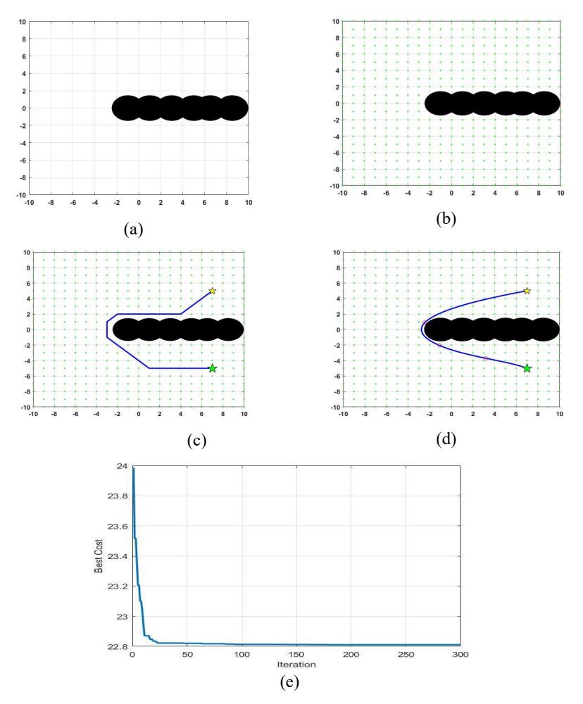
Figure 3 Run of first suggested mobile robot environment.
Figure 4 shows the run of the second suggested mobile robot environment containing a variety of static obstacles. In Figure 3(a), the black circles indicate the obstacle space in the second mobile robot environment. In Figure 4(b), the green points indicate the free space in the second mobile robot environment.
Figure 4(c) shows the free-collision shortest path of the mobile robot from the start point (-8, 7) to the goal point (-5, 1) with a fitness function cost equal to 30.313. While Figure 4(d) shows the optimal smooth path generated by the proposed method, with a fitness function cost equal to 28.5331. Figure 4(e) shows the alteration of path cost along the algorithm's iterations.
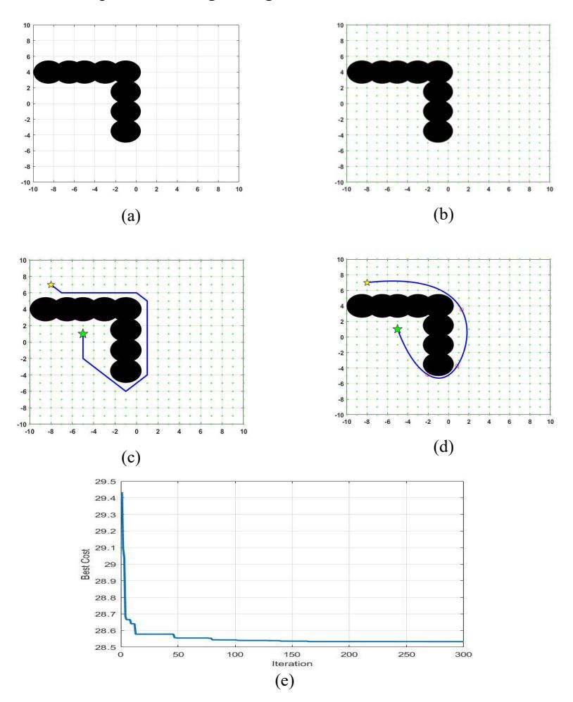
Figure 4 Run of second suggested mobile robot environment.
The proposed method was also applied to test another suggested, Figure 5 shows the run of the third simulated mobile robot environment containing a variety of static obstacles. In Figure 5(a), the black circles indicate the obstacle space in the suggested mobile robot environment. In Figure 5(b), the green points indicate the free space in the suggested mobile robot environment.
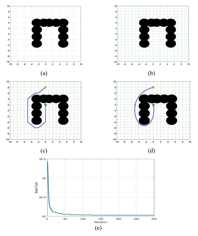
Figure 5 Run of Third Suggested Mobile Robot Environment.
Figure 5(c) shows the free-collision shortest path of the mobile robot from the start point (0, 8) to the goal point (0, 2) with a fitness function cost equal to 27.313. Figure 5(d) shows the optimal smooth path generated by the proposed method, with a fitness function cost equal to 25.03. Figure 5(e) shows the alteration of path cost along the algorithm's iterations.
Figure 6 shows the run of the suggested mobile robot environment containing a variety of static obstacles. In Figure 6(a), the black circles indicate the obstacle
space of the suggested mobile robot environment. In Figure 6(b), the green points indicate the free space in the suggested mobile robot environment. Figure 6(c) indicates the free-collision shortest path of the mobile robot from the start point (-3, -8) to the goal point (3, -8), with a fitness function cost equal to 44.142. Figure 6(d) shows the optimal smooth path generated by the proposed method, with a fitness function cost equal to 40.815. Figure 6(e) illustrates the alteration of path cost along the algorithm's iterations.
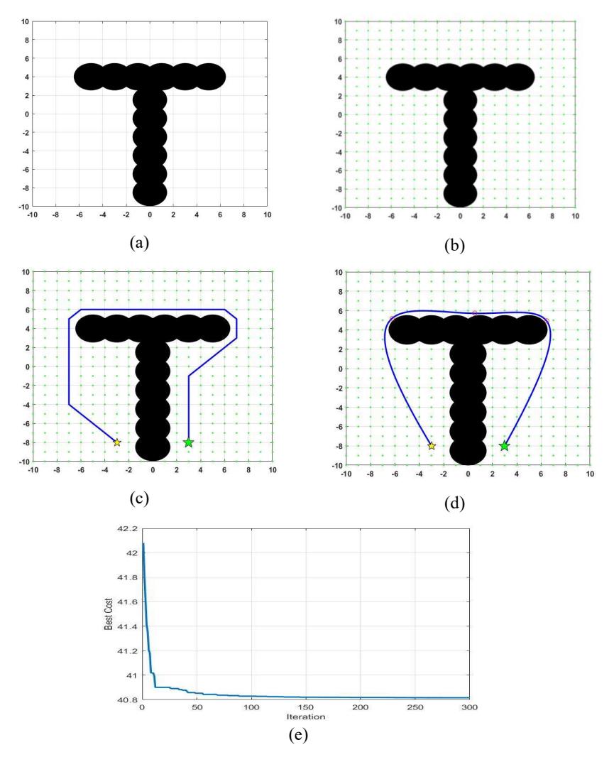
Figure 6 Run of the fourth suggested mobile robot environment.
The proposed method was also applied to test another suggested, Figure 7 shows the run of the fifth simulated mobile robot environment containing a variety of static obstacles. In Figure 7(a), the black circles indicate the obstacles space of suggested mobile robot environment. In Figure 7(b), the green points indicate the free space in the suggested mobile robot environment. Figure 7(c) indicates the free-collision shortest path of the mobile robot from the start point (-9, -8) to the goal point (8, -3), with a fitness function cost equal to 36.485. Figure 7(d) represents the optimal smooth path generated by the proposed method, with a fitness function cost equal to 33.89. Figure 7(e) shows the alteration of path cost along the algorithm's iterations.
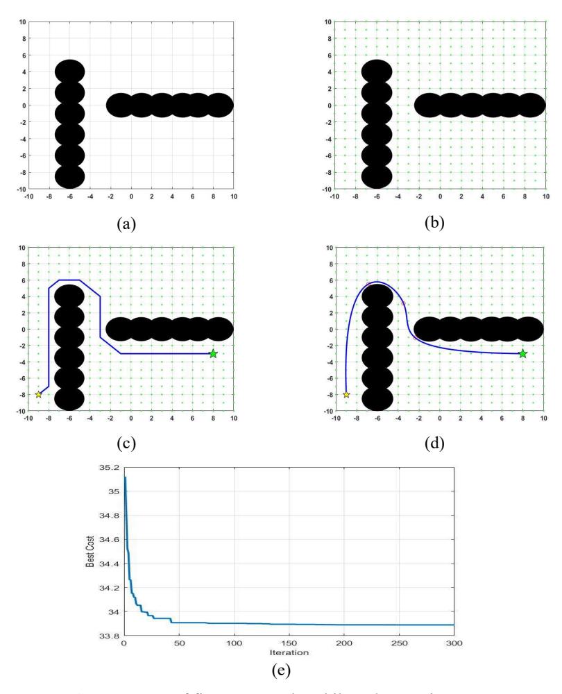
Figure 7 Run of five Suggested Mobile Robot Environment.
Figure 8 represents the run of the suggested mobile robot environment that contains of a variety of static obstacles. In Figure 8(a), the black circles indicate the obstacle space of suggested mobile robot environment. In Figure 8(b), the green points indicate the free space of suggested mobile robot environment. Figure 8(c) shows the free-collision shortest path of the mobile robot from the start point (0, 7) to the goal point (-3, -8), with a fitness function cost equal to 17.071. Figure 8(d) shows the optimal smooth path generated by the proposed method, with a fitness function cost equal to 16.154. Figure 8(e) shows the alteration of path cost along the algorithm's iterations.
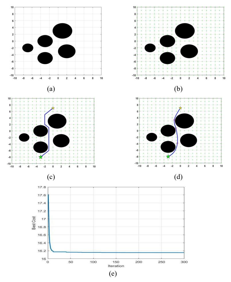
Figure 8 Run of Six Suggested Mobile Robot Environment.
The proposed method was also applied to test another suggested mobile robot environment, as represented in Figure 9 In Figure 9(a), the black circles indicate the obstacle space of suggested mobile robot environment. In Figure 9(b), the green points indicate the free space of suggested mobile robot environment. Figure 9(c) shows the free-collision shortest path of the mobile robot from the start point (6, 8) to the goal point (-3, -9), with a fitness function cost equal to 20.727. Figure 9(d) shows the optimal smooth path generated by the proposed method, with a fitness function cost equal to 19.368. Figure 9(e) shows the alteration of path cost along the algorithm's iterations.
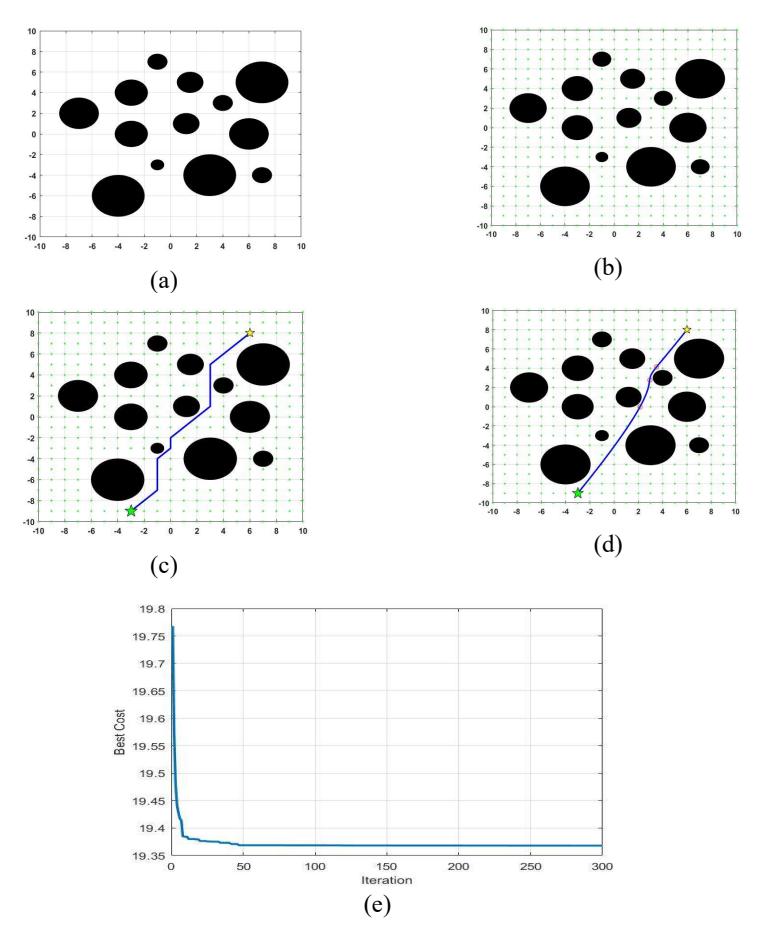
Figure 9 Run of Seven Suggested Mobile Robot Environment.
Table 1 explains the results of all cases that were tested in the suggested environments.
| Environment | Test point | A* aast | Eineffer each | ||
|---|---|---|---|---|---|
| Start | Goal | A* cost | Firefly cost | ||
| 1 | 7,5 | 7,-5 | 25.313 | 22.811 | |
| 2 | -8,7 | -5,1 | 30.313 | 28.5331 | |
| 3 | 0,8 | 0,2 | 27.313 | 25.03 | |
| 4 | -3,-8 | 3,-8 | 44.142 | 40.815 | |
| 5 | -9,-8 | 8,-3 | 36.485 | 33.89 | |
| 6 | 0,7 | -3,-8 | 17.071 | 16.154 | |
| 7 | 6,8 | -3,-9 | 20.7279 | 19.368 | |
Table 1 Tested Results of Run of suggested mobile robot environments.
Table 2 presents a basic comparison with the results from another published paper in terms of the number of iterations of the best result found and the cost.
| Table 2 | Comparison | between the | e method o | f [20] ar | nd the pro | oposed method. |
|---|
| Environment | Test J | ooint | - Firefly cost of | Firefly cost based on the A* algorithm |
|---|---|---|---|---|
| Start | Goal | [20] | ||
| 1 | 2,-1 | 1,-8 | 25.473 | 25.442 |
| 2 | 3,7 | -3,7 | 38.887 | 37.953 |
| 3 | 8,8 | -8,4 | 34.05 | 34.186 |
| 4 | 5,-8 | -6,8 | 20.071 | 20.0062 |
| 5 | -8,-6 | 8,2 | 20.773 | 19.8418 |
The obtained comparison result shows the superiority of the method proposed in this paper in finding the shortest path.
5 Conclusion
Optimal path planning is an important concern in the navigation of autonomous mobile robots, which consists of finding an optimal path according to some criteria, such as distance, time, and energy. Distance or time are the most commonly adopted criteria. Nature-inspired heuristic algorithms are considered powerful in solving modern global optimization problems, especially when dealing with NP-hard optimization, such as the traveling salesman problem and path planning. In this study, a swarm intelligence approach (the firefly algorithm) inspired by biological behavior was applied to the robot path optimization problem. The two essential functions of the proposed improvement are used to find the free space in a mobile robot environment and then generates the freecollision shortest path from its start to goal point based on the firefly algorithm.
The A* algorithm is used to create the shortest path from start to goal point by avoiding all obstacles. The principle of operation of proposed A* algorithm is locally planning the shortest path within the free space until the goal point is reached. The generated path from the implementation of the A* algorithm is considered the best shortest path. The proposed smooth trajectory design was based on iterative random selection and interpolation of the intermediate via points on the A* shortest path until achieving a possible smooth path. The firefly algorithm is used to generate and rapidly converges a specific number of intermediate via points.
Cubic polynomial trajectory equations are applied for producing the corresponding smooth trajectory within a specific time. Modeling the run of the proposed method within several simulated environments with varying degrees of complexity showed that obstacles were successfully avoided, the free collision optimal path is efficiently planned, and the mobile robot could smoothly follow the optimal path.