
1 Introduction
Directivity and desired radiation patterns are two of the main targeted improvements in antenna array performance [1]. By focusing on the desired radiation pattern, the requirements for the suppression of the sidelobe level (SLL) and the width of main lobe (WML) are two metric performance factors in antenna array design based on the use cases [2,3]. A well-known method for performance optimization of antenna arrays is the power-weighted method, which has been investigated over the last several decades [4,5]. SLL suppression in antenna arrays using the power-weighted method is commonly done by distributing
weighted power to each element based on a set of coefficients. The ordering of the power-weight allocation is executed by engaging a different impedance of the transmission line for every element, so that it provides weighted current and power alike [6].
The application of a window function as weighting coefficient has been discussed in some references from the 1980s [7,8]. Besides a Chebyshev function, other functions such as a Kaiser function and a Blackman function are also applicable to meet the performance metric requirement. Both have been declared as two window functions that can attain improved SLL suppression in antenna arrays [9- 12]. Unfortunately, the research on the radiation pattern properties in powerweighted antenna arrays with a linear arrangement based on both functions is limited. Previous investigations are reported in [13,14]. The main motivation for investigating the possibility of using other window functions is to have a promising approach for application in power-weighted antenna array designs where slight differences in degree of elevation and azimuth beam widths are very important [2,3]. An analytical approach using a mathematical formulation in developing a design model for a certain type of antenna and optimizing a beamformer device with a required pattern has been described as reliable in [15,16].
In order to have more choice in implementing power-weighted antenna array designs, application of a Kaiser function is an interesting but challenging alternative. Some benefits of applying a Kaiser function are that it provides broader main lobes in the radiation pattern and comparable flexibility in SLL suppression with a Chebyshev function. However, a study of Kaiser function parameter determination using an analytical approach on power-weighted antenna arrays is still required as part of the investigations prior to simulation and measurement. The exploration of the radiation pattern properties of Kaiser and Blackman functions applied in power-weighted antenna arrays with a linear arrangement are executed using a mathematical formulation. The radiation patterns of Kaiser and Blackman functions tend to be relatable for a distinct value of the Kaiser function's parameter β.
A report of the analytical comparison of radiation characteristics that focused on a Blackman function and its comparison with a Kaiser function was compiled in [17]. These two window functions also seem to have enhanced the WML when compared to a Chebyshev function and they are useful for broadside antenna array designs [4]. The possibility of applying a Kaiser function in an antenna array was explored by further investigation of its features as well as implementing Blackman and Chebyshev functions for comparison. Since the β parameter is used in obtaining the set of coefficients based on the targeted SLL [18], the Kaiser function has similar flexibility as the Chebyshev function. This is considered one of the advantages of Kaiser function application in power-weighted antenna arrays. The determination of the β parameter in the design of antenna arrays based on a Kaiser function is informative. In this study, the terminology of determination includes calculation, optimization, and validation. The focus of this study was the observation of radiation patterns without considering other antenna parameters. Gain, polarization, and bandwidth were not the focus of the investigation. There are also predictable drawbacks in Kaiser function implementation, such as a bigger β, resulting in the first and last weighting values getting closer to 0, and there being less implementation report. This makes implementation in a prototype very challenging. Several arrangements of linear antenna arrays based on Kaiser, Blackman, and Chebyshev functions were executed to look into the flexibility of the Kaiser function in relation to the targeted SLL and the accuracy of its β.
2 Antenna Array Arrangement
A geometric model implementing the power-weighted method in an antenna array design is illustrated in Figure 1, with N as the total number of elements and d as the distance between elements. This model was developed based on the geometry of a linear antenna array with non-uniform amplitude distribution and uniform distance between elements [19], as well as implementing some essential aspects of array pattern synthesis [20 and power-weighted antenna array designs [21,22]. The application of a Kaiser function in the power-weighted method for linear antenna arrays was first carried out by determining the desired SLL target, the working frequency, the number of antenna array elements, and the type of antenna and feeding network used.
Having determined these important parameters, the basic idea of applying the power-weighted method is to ensure that the power delivered to each antenna element has been weighted or multiplied by a coefficient according to the weighting function used. This is done by weighting the amplitude of the current that feeds each element of the antenna array. Therefore, the feeding network must be designed in such a way that the power distributed to each element corresponds to the weighting coefficient used. For analysis purposes, a spherical coordinate was used instead of a Cartesian coordinate, where is the polar angle, ranging from 0 to , and started from the -axis, while is the azimuth angle, ranging from 0 to 2, and measured from the -axis.
3 Array Factor Pattern
In general, the array factor is a function of a number of elements, geometrical arrangements, distance, relative magnitudes, and relative phases [23]. The antenna array design, which has the same amplitude, phase, and distance for every
element, will have a noncomplex form of the array factor. Since the array factor is independent from the directional characteristics of the radiating elements, it can be expressed by displacing the real elements with isotropic point sources. The total field of the real antenna array is obtained by multiplying the singular element fields at a picked reference point with the array factor.
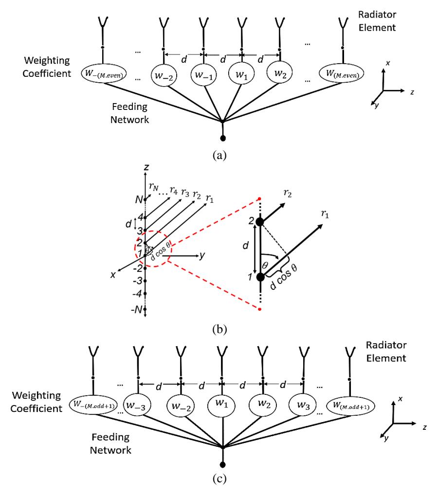
Figure 1 Configuration of the antenna array model in a linear arrangement. (a) Even N elements, (b) arrangement geometry of N elements with distance d between elements along the z-axis [23], (c) odd N elements.
The radiated far-field zone of an antenna array of identical elements, E (total), is equal to the product of the field of a singular element at the point of origin, E
(single element at reference point), and its array factor. Eq. (1) is specified as a multiplication pattern for an array with identical elements:
\[E(total) = [E(single\ element\ at\ reference\ point)] \times [array\ factor]\] (1)
This multiplication pattern is valid for arrays with any number of identical elements; it has a similar pattern and is oriented in the same direction [23,24]. Since the array factor can be ascertained, this approach is useful for gaining insight into predicting the radiation patterns of antenna array designs. Therefore, several assumptions are necessary to predict the overall radiation pattern of the antenna array using the array factor. These assumptions include that the isotropic elements are identical and that the distance between elements is uniform [23].
Moreover, the implication of mutual coupling is also neglected, since the distance between elements equals more than \(\lambda/2\) while the range of the number of elements is quite extended, \(7 \le N \le 178\). Based on these assumptions, the resulted properties when applying a Kaiser function in a power-weighted antenna array were explored. The range of number of elements \(7 \le N \le 178\) was chosen to represent some odd and even numbers of elements in the range of 0 to 200. The explored values of N were 7, 8, 77, 78, 107, 108, 177, 178. This wide range was chosen to represent antenna arrays with small and large numbers of elements. The process of exploration consisted of three main procedures. The first involved inputting some variables into the calculation process, such as operation frequency, number of elements, and distance between elements. The second involved calculating the array factor, while the last involved analyzing the array factor figures. An antenna array in a linear arrangement with N elements positioned on the z-axis is shown in Figure 1, where the array factor can be expressed as follows [23]:
\[AF = \sum_{n=1}^{N} w_n e^{j(n-1)(kd \cos \gamma + \delta)}\] (2)
where \(w_n\) is the weighting coefficient of the array elements, also known as the excitation coefficient [4]; \(\delta\) is the progressive phase excitation between elements; n is the element number; k is the wave vector, and \(\gamma\) is the angle between the axis of the array (z-axis) and the radial vector from the origin to the point of observation.
When the elements are placed along the z-axis, the angle \(\gamma\) is equal to angle \(\theta\), as shown in Figure 1. An antenna array with a linear arrangement of an even number of isotropic elements \(N=2M_{even}\), where \(M_{even}\) is an integer, is placed symmetrically along the z-axis. By assuming that the amplitude excitation is symmetrical to the origin, the array factor for a non-uniform amplitude broadside array can be expressed as follows [23]:
\[(AF)_{2Meven} = \sum_{n=1}^{Meven} w_n \cos \left[ \frac{(2n-1)}{2} kd \cos \theta \right]\] (3)
If the total number of elements is odd, \(N = 2M_{odd} + 1\), where \(M_{odd}\) is an integer, the array factor can be expressed as follows [22]:
\[(AF)_{2Modd+1} = \sum_{n=1}^{Modd+1} w_n \cos[(n-1) kd \cos \theta]\] (4)
For generalization purposes, Eq. (3) and (4) can be rewritten as Eq. (5) and (6), respectively,
\[(AF)_{2Meven}(even) = \sum_{n=1}^{Meven} w_n \cos[(2n-1)u]\] (5)
\[(AF)_{2Modd+1}(odd) = \sum_{n=1}^{Modd+1} w_n \cos[2(n-1)u]\] (6)
where,
\[u = \frac{\pi d}{\lambda} \cos \theta \tag{7}\]
It is noted that u corresponds to the physical space between the radiators. By properly selecting \(w_n\), the coefficient can be employed to approximate diverse desired radiation patterns.
4 Kaiser Function-based Weighting Coefficient
The Kaiser function is specified as the Kaiser-Bessel function [18]. This particular window function has an extra degree of flexibility, as it is able to vary the main lobe beam width and the sidelobe ratio [24]. The Kaiser function-based weighting coefficient is written as follows [7,8]:
\[w(n) = \frac{{}^{1I_{0Bessel}} \left(\beta \sqrt{1 - \left(\frac{n}{N/2}\right)^2}\right)}{I_{0Bessel}(\beta)} - M_{odd} + 1 \le n \le M_{odd} + 1 \text{ or }\]\[-M_{even} \le n \le M_{even}\](8)
where \(I_{0Bessel}\) is the first type of zero-th order modified Bessel functions, and \(\beta\) is the Kaiser function parameter obtained from the empirical relationship in Eq. (9), with A as the targeted SLL [17]:
\[\beta = \begin{cases} 0.1102(A - 8.7) & A > 50\\ 0.5842(A - 21)^{0.4} + 0.07886(A - 21) & 21 \le A \le 50\\ 0 & A < 21 \end{cases}\](9)
The Kaiser function can also approximate a number of other windows by varying its window shape parameter, \(\alpha\) [23]. The Kaiser function parameter used in this paper is \(\beta\), where the relationship between \(\beta\) and \(\alpha\) is \(\beta = \pi \alpha\) [7, 8]. The Kaiser function parameter will direct the trade-off between the main lobe beam width and the sidelobe ratio [7,25]. A different \(\beta\) value will yield a different set of coefficients in designing the power-weighted antenna array. Comparatively, the Blackman function in a planar and linear antenna array has a fairly broad main
lobe [12,13]. Weighting coefficients based on the Blackman function are expressed in [7,26]. Moreover, a pattern with high SLL suppression and a narrow WML can be obtained through the power-weighted method based on the Chebyshev function [27]. The application of a Chebyshev function as a weighting coefficient is one of the most popular choices to achieve a narrow beam width with a specified targeted SLL. In contrast, for a specified beam width, all the sidelobes of a Chebyshev-based array are of equal height at the lowest level [1].
5 Radiation Pattern of Antenna Array and Its Comparison
Investigation of the power-weighted antenna array based on Kaiser and Blackman functions with a linear arrangement was conducted by varying N and d [13,14]. In this investigation, the specific patterns were the elevation patterns, or the Eplane, in co-polarization. The radiation patterns of the power-weighted antenna array based on the Blackman function with a linear arrangement are reported in [13]. The radiation patterns of the power-weighted antenna array based on the Kaiser function with a linear arrangement for even and odd numbers of element variations and a constant d of /. are reported in [14]. The results indicated that the increase of notably impacted the WML, causing it to become narrower, and the increase of d affected a narrower WML. The investigation of some variable variations in the application of a Chebyshev function are reported in [28]. Similar conditions between Kaiser, Blackman, and Chebyshev functions take place when there is variation of with a constant N.
A synthesizing process was conducted throughout the study by configuring the SLL using the Blackman function and referring the obtained SLL to determine A and β with Eq. (9) in the Kaiser function. The original values of β, which were obtained from Eq. (9), yielded different values of the obtained SLL. Thus, an adjustment of β was necessary to achieve a similar targeted SLL. The adjustment of β was executed by comparing between the Kaiser and the Blackman function, as plotted in Figure 4, where the optimized β value was 9.5. Increasing β will give a broader main lobe and will decrease the amplitude of the sidelobes, increasing the sidelobe attenuation [7]. The Blackman function had a broader WML when compared to the Chebyshev function in the antenna array with an N of 8 [13] and also the one with an N of 80, as plotted in Figure 2. The outcomes show that for an N of 8, the Blackman function had a half power beam width (HPBW) of 42°, and the Chebyshev function had an HPBW of 32°. Meanwhile, for an N of 80, the Blackman function had an HPBW of 4°, and the Chebyshev function had an HPBW of 3.2°. By using the Kaiser function, a broader main lobe can be achieved, similar to the Blackman function, which is also more flexible and adjustable in relation to the targeted SLL, similar to the Chebyshev function. The results of applying the Kaiser function with an N of 80 and an HPBW of 3.6°, are depicted in Figure 3.
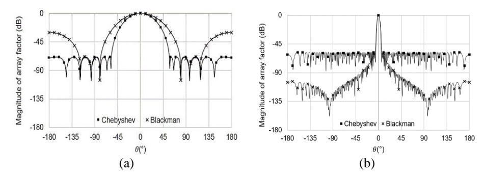
Figure 2 Radiation patterns of power-weighted antenna array based on Chebyshev and Blackman functions, with targeted SLL = 68.8 dB for N= 8 and SLL = 58.12 dB for N = 80, (a) N= 8, (b) N= 80.
Comparing the specific β values, the radiation pattern of the Kaiser function is similar to that of the Chebyshev function but with a wider main lobe. Figure 4 shows the radiation pattern comparison of the power-weighted antenna array based on the Kaiser and Blackman functions with an arrangement N of 8, a d of λ/1.5, a presumed SLL of 68.8 dB, and a β of 6.623 [13].
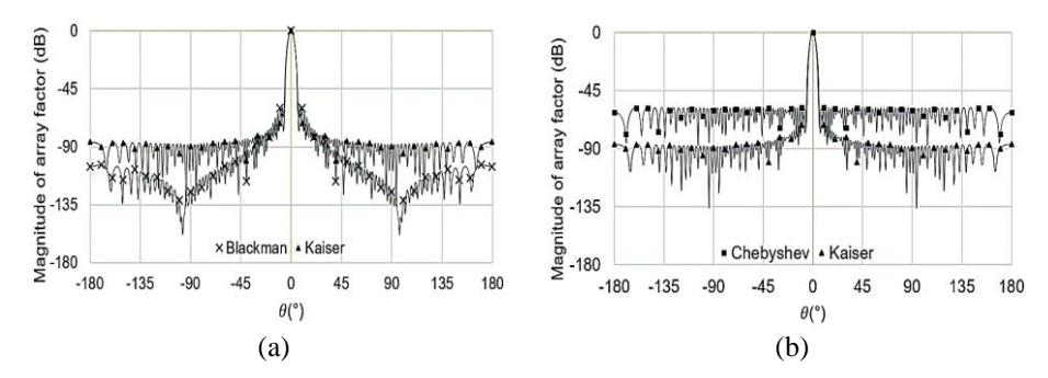
Figure 3 Radiation patterns of power-weighted antenna array based on Kaiser and Blackman function, with targeted SLL = 58.12 dB, N = 80 and β = 7.98, (a) Blackman versus Kaiser function, (b) Chebyshev versus Kaiser function.
Figure 4 plots the comparison of the radiation patterns of a power-weighted antenna array based on the Kaiser, Blackman, Chebyshev window functions, and a uniform distribution. Specifically, the comparison of the WML and SLL of the Kaiser, Blackman, and Chebyshev functions showed similar SLL results. The WML of the Chebyshev function was narrower compared to the Kaiser and Blackman functions. Additionally, the comparison with a uniform distribution was used as the baseline. The comparison of Kaiser function application in a linear antenna array with a uniform distribution as baseline is shown in Figure 6.
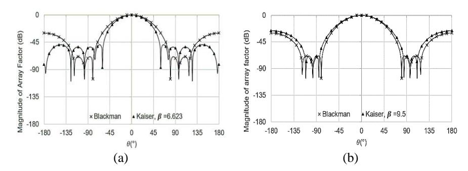
Figure 4 Radiation patterns of power-weighted antenna array based on Blackman and Kaiser functions, with N = 8 and SLL = 68.8 dB, (a) β = 6.623, (b) β optimization, β= 9.5.
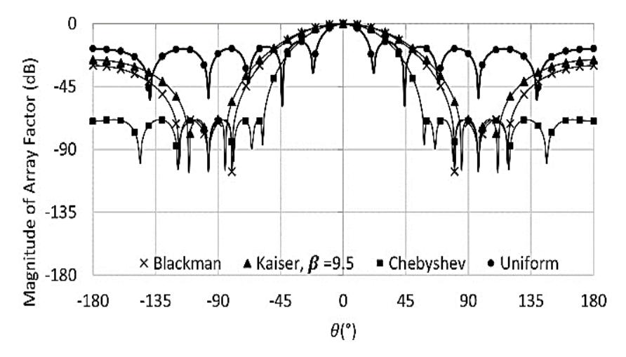
Figure 5 Radiation patterns of power-weighted antenna array based on Blackman, Kaiser, Chebyshev functions and a uniform distribution, with N= 8, SLL= 68.8 dB, and β= 9.5.
A uniform distribution is also known as a rectangular window and is unity over the observation interval [7]. The highest SLL by using a uniform distribution was 13 dB, so the β value for 13 dB targeted SLL according to Eq. (9) was 0. From Figure 6 (a) and (b), the comparison not only clearly shows the similarity of the SLL but also the similarity of the WML between the Kaiser function and the uniform distribution, as well as the improvement of SLL performance when using higher values of β. For β = 0, the SLL suppression was 13 dB, for β= 1.5 the SLL suppression was 17 dB, and for β= 3 the SLL suppression was 27 dB. This confirms the ability of the Kaiser function to approximate another window function by varying its β value and its flexibility in achieving stronger SLL suppression.
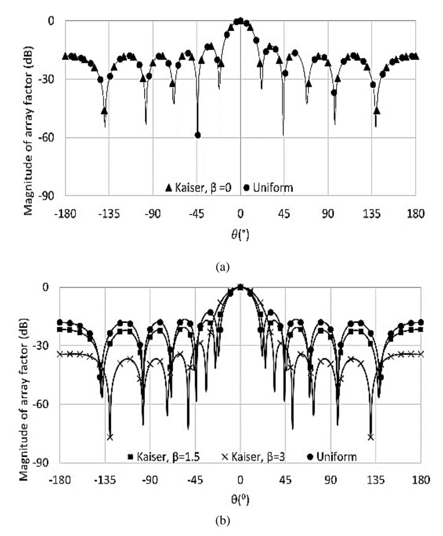
Figure 6 Radiation patterns of power-weighted antenna array based on Kaiser functions and uniform distribution, N= 8, (a) Kaiser β= 0, (b) Kaiser β= 1.5 & 3.
6 Optimization and Validation of the Kaiser Function Parameter (β)
From the aforementioned discussion, it can be decided that since the β obtained from Eq. (9) yielded a different SLL value, an adjustment is needed to achieve an accurate SLL value. Table 1 illustrates the targeted SLLs of 25 dB, 35 dB and 45 dB and the impact of N variation with the same β value.
Table 1 Original with N variations in constant targeted SLL.
| N | 25 dB, 𝜷=1.333 | Targeted SLL (dB) 35 dB, 𝜷=2.783 Obtained SLL (dB) | 45 dB, 𝜷=3.975 |
|---|---|---|---|
| 5 | 15.94 | 23.57 | 23.08 |
| 10 | 16.07 | 25.55 | 33.82 |
| 15 | 15.89 | 23.02 | 28.16 |
| 25 | 15.82 | 22.82 | 28.98 |
| 30 | 16.10 | 23.36 | 31.17 |
| 35 | 15.84 | 22.77 | 29.26 |
| 40 | 15.83 | 23.13 | 30.79 |
| 45 | 15.78 | 22.72 | 29.43 |
| 50 | 15.81 | 23.00 | 30.59 |
| 55 | 15.76 | 22.67 | 29.49 |
| 60 | 15.78 | 22.94 | 30.47 |
| 65 | 15.75 | 22.65 | 29.55 |
| 70 | 15.78 | 22.87 | 30.38 |
| 75 | 15.75 | 22.64 | 29.58 |
| 80 | 15.76 | 22.82 | 30.33 |
| 85 | 15.74 | 22.61 | 29.64 |
| 90 | 15.79 | 22.75 | 30.23 |
| 95 | 15.74 | 22.61 | 29.68 |
| 100 | 15.76 | 22.74 | 30.18 |
| 105 | 15.74 | 22.64 | 29.65 |
| 110 | 15.76 | 22.75 | 30.15 |
| 115 | 15.74 | 22.58 | 29.74 |
| 120 | 15.77 | 22.70 | 30.24 |
| 125 | 15.77 | 22.58 | 29.68 |
| 130 | 15.76 | 22.71 | 30.17 |
| 135 | 15.73 | 22.72 | 29.72 |
| 140 | 15.76 | 22.70 | 30.15 |
| 145 | 15.79 | 22.57 | 29.75 |
| 150 | 15.73 | 22.71 | 30.05 |
| 155 | 15.80 | 20.64 | 29.70 |
| 160 | 15.73 | 22.66 | 30.12 |
| 165 | 15.81 | 22.69 | 29.70 |
| 170 | 15.73 | 22.63 | 30.14 |
| 175 | 15.80 | 22.72 | 29.75 |
| 180 | 15.76 | 22.63 | 30.09 |
| 185 | 15.74 | 22.66 | 29.77 |
| 190 | 15.86 | 22.67 | 30.12 |
| 195 | 15.72 | 22.57 | 29.74 |
| 200 | 15.74 | 22.82 | 30.24 |
The investigation of an appropriate β value for different values of A was run by focusing on the second range Eq. (9). The accuracy of the β value is very important to achieve accurate SLL suppression, which will significantly affect the SLL error percentage. The second-range Eq. (9) and the adjustment of the β parameter for an N of 7, 8, 77, 78, 107, 108, 177, 178 were used to calculate the data in Tables 2 to 5. From this data, the optimum β value was analytically obtained.
Table 2 values based on targeted SLL A and its results in a power-weighted antenna array based on the Kaiser function, N=7 and N=8.
| Targeted SLL(dB) | β | Obtained SLL(dB) | Optimized β | Revised Obtained SLL (dB) | β error percentage (%) | ||||
|---|---|---|---|---|---|---|---|---|---|
| N= 7 | N = 8 | N = 7 | N = 8 | N = 7 | N= 8 | N= 7 | N = 8 | ||
| 21 | 0 | 12.80 | 12.79 | 2.30 | 2.11 | 21.01 | 21.06 | 100 | 100 |
| 22 | 0.66 | 13.58 | 13.61 | 2.50 | 2.24 | 22.05 | 22.07 | 73 | 70 |
| 23 | 0.93 | 14.35 | 14.40 | 2.72 | 2.35 | 23.05 | 22.97 | 66 | 60 |
| 24 | 1.14 | 15.10 | 15.22 | 2.98 | 2.48 | 23.99 | 24.07 | 62 | 54 |
| 25 | 1.33 | 15.90 | 16.11 | 3.50 | 2.59 | 24.99 | 25.03 | 62 | 49 |
| 26 | 1.51 | 16.73 | 17.03 | 6.20 | 2.69 | 26.05 | 26.06 | 76 | 44 |
| 27 | 1.67 | 17.55 | 18.01 | 9.20 | 2.82 | 27.00 | 27.04 | 82 | 41 |
| 28 | 1.82 | 18.35 | 18.95 | 11.10 | 2.93 | 28.02 | 27.98 | 84 | 38 |
| 29 | 1.97 | 19.19 | 20.01 | 12.20 | 3.05 | 29.17 | 28.99 | 84 | 35 |
| 30 | 2.12 | 20.04 | 21.15 | 12.80 | 3.18 | 30.01 | 30.03 | 83 | 33 |
| 31 | 2.26 | 20.76 | 22.24 | 13.40 | 3.32 | 31.00 | 31.06 | 83 | 32 |
| 32 | 2.39 | 21.49 | 23.31 | 13.95 | 3.47 | 32.08 | 32.04 | 83 | 31 |
| 33 | 2.52 | 22.14 | 24.41 | 14.35 | 3.65 | 32.99 | 33.02 | 82 | 31 |
| 34 | 2.65 | 22.76 | 25.54 | 14.80 | 3.90 | 34.12 | 34.10 | 82 | 32 |
| 35 | 2.78 | 23.29 | 26.71 | 15.20 | 4.20 | 35.29 | 35.04 | 82 | 34 |
| 36 | 2.91 | 23.79 | 27.81 | 15.43 | 4.52 | 36.02 | 35.96 | 81 | 36 |
| 37 | 3.03 | 24.14 | 28.83 | 15.72 | 4.83 | 37.04 | 36.95 | 81 | 37 |
| 38 | 3.16 | 24.46 | 29.88 | 15.98 | 5.15 | 38.05 | 38.26 | 80 | 39 |
| 39 | 3.28 | 24.69 | 30.77 | 16.20 | 5.30 | 38.98 | 38.99 | 80 | 38 |
| 40 | 3.4 | 24.90 | 31.66 | 16.42 | 5.49 | 40.01 | 40.01 | 79 | 38 |
| 41 | 3.51 | 25.00 | 32.26 | 16.63 | 5.70 | 41.07 | 41.29 | 79 | 38 |
| 42 | 3.63 | 25.09 | 32.92 | 16.80 | 5.82 | 42.04 | 42.15 | 78 | 38 |
| 43 | 3.75 | 25.15 | 33.48 | 16.96 | 5.93 | 42.99 | 42.92 | 78 | 37 |
| 44 | 3.86 | 25.24 | 33.92 | 17.20 | 6.08 | 44.63 | 44.07 | 78 | 36 |
| 45 | 3.98 | 25.22 | 34.36 | 17.28 | 6.19 | 45.21 | 45.00 | 77 | 36 |
| 46 | 4.09 | 25.22 | 34.74 | 17.40 | 6.30 | 46.16 | 45.96 | 77 | 35 |
| 47 | 4.2 | 25.24 | 35.04 | 17.50 | 6.42 | 47.01 | 47.08 | 76 | 35 |
| 48 | 4.31 | 25.28 | 35.34 | 17.60 | 6.51 | 47.93 | 48.05 | 75 | 34 |
| 49 | 4.42 | 25.26 | 35.75 | 17.70 | 6.62 | 48.91 | 49.09 | 75 | 33 |
| 50 | 4.53 | 25.28 | 35.99 | 17.80 | 6.72 | 49.99 | 50.12 | 75 | 33 |
Table 3 values based on targeted SLL A and its results in a power-weighted antenna array based on Kaiser function, N= 77 and N = 78.
| Targeted SLL(dB) | β | Obtained SLL(dB) | Optimized β | Revised Obtained SLL (dB) | β error percentage (%) | ||||
|---|---|---|---|---|---|---|---|---|---|
| N= 77 | N = 78 | N= 77 | N = 78 N = 77 | N= 78 | N= 77 | N = 78 | |||
| 21 | 0 | 13.28 | 13.28 | 2.50 | 2.48 | 21.08 | 21.10 | 100 | 100 |
| 22 | 0.66 | 13.90 | 13.89 | 2.68 | 2.63 | 22.05 | 22.00 | 75 | 75 |
| 23 | 0.93 | 14.51 | 14.51 | 2.85 | 2.82 | 23.05 | 23.06 | 67 | 67 |
| 24 | 1.14 | 15.14 | 15.18 | 3.03 | 2.99 | 24.04 | 24.05 | 62 | 62 |
| 25 | 1.33 | 15.71 | 15.75 | 3.20 | 3.16 | 25.01 | 25.17 | 58 | 58 |
| 26 | 1.51 | 16.41 | 16.44 | 3.40 | 3.32 | 26.19 | 26.07 | 56 | 55 |
| 27 | 1.67 | 17.11 | 17.10 | 3.55 | 3.48 | 27.11 | 27.10 | 53 | 52 |
| 28 | 1.82 | 17.71 | 17.75 | 3.72 | 3.63 | 28.09 | 28.04 | 51 | 50 |
| 29 | 1.97 | 18.42 | 18.49 | 3.89 | 3.78 | 29.08 | 29.03 | 49 | 48 |
| 30 | 2.12 | 19.11 | 19.19 | 4.00 | 3.93 | 29.73 | 30.02 | 47 | 46 |
Table 3 Continued. \(\beta\) values based on targeted SLL A and its results in a powerweighted antenna array based on the Kaiser function, N = 77 and N = 78.
| Targeted SLL(dB) | β | Obtained SLL(dB) | Optimized β | Revised Obtained SLL (dB) | β error percentage (%) | ||||
|---|---|---|---|---|---|---|---|---|---|
| N= 77 | N= 78 | N= 77 | N= 78 | N= 77 | N= 78 | N= 77 | N= 78 | ||
| 31 | 2.26 | 19.83 | 19.93 | 4.22 | 4.10 | 31.10 | 31.12 | 47 | 45 |
| 32 | 2.39 | 20.58 | 20.60 | 4.41 | 4.25 | 32.10 | 32.11 | 46 | 44 |
| 33 | 2.52 | 21.19 | 21.32 | 4.58 | 4.38 | 33.10 | 33.01 | 45 | 42 |
| 34 | 2.65 | 21.89 | 22.05 | 4.75 | 4.53 | 34.04 | 34.01 | 44 | 41 |
| 35 | 2.78 | 22.62 | 22.81 | 4.95 | 4.69 | 35.11 | 35.06 | 44 | 41 |
| 36 | 2.91 | 23.43 | 23.57 | 5.14 | 4.84 | 36.10 | 36.06 | 43 | 40 |
| 37 | 3.03 | 24.04 | 24.30 | 5.32 | 4.98 | 36.99 | 37.13 | 43 | 39 |
| 38 | 3.16 | 24.79 | 25.08 | 5.55 | 5.12 | 38.14 | 38.00 | 43 | 38 |
| 39 | 3.28 | 25.50 | 25.84 | 5.77 | 5.27 | 39.06 | 39.04 | 43 | 38 |
| 40 | 3.4 | 26.19 | 29.38 | 6.00 | 5.45 | 40.05 | 40.22 | 43 | 38 |
| 41 | 3.51 | 26.86 | 28.41 | 6.24 | 5.60 | 41.08 | 41.22 | 44 | 37 |
| 42 | 3.63 | 27.55 | 41.22 | 6.53 | 5.70 | 42.08 | 41.91 | 44 | 36 |
| 43 | 3.75 | 28.28 | 28.86 | 6.80 | 5.87 | 43.03 | 43.16 | 45 | 36 |
| 44 | 3.86 | 28.90 | 29.54 | 7.16 | 6.00 | 44.09 | 43.99 | 46 | 36 |
| 45 | 3.98 | 29.63 | 30.38 | 7.55 | 6.17 | 45.05 | 45.16 | 47 | 36 |
| 46 | 4.09 | 30.25 | 31.05 | 8.05 | 6.30 | 46.08 | 46.02 | 49 | 35 |
| 47 | 4.2 | 30.90 | 31.80 | 8.79 | 6.39 | 47.11 | 46.75 | 52 | 34 |
| 48 | 4.31 | 31.53 | 32.52 | 10.20 | 6.59 | 48.04 | 48.03 | 58 | 35 |
| 49 | 4.42 | 32.15 | 33.25 | 11.00 | 6.73 | 48.24 | 49.04 | 60 | 34 |
| 50 | 4.53 | 32.79 | 34.01 | 12.50 | 6.86 | 48.34 | 49.97 | 64 | 34 |
Table 4 \(\beta\) values based on targeted SLL A and its results in a power-weighted antenna array based on the Kaiser function, N=107 and N=108.
| Targeted SLL(dB) | β | Obtained SLL(dB) | Optimized β | Revised Obtained SLL (dB) | β error percentage (%) | ||||
|---|---|---|---|---|---|---|---|---|---|
| , , | N = 107 | N= 108 | N= 107 | N= 108 | N= 107 | N= 108 | N= 107 | N= 108 | |
| 21 | 0 | 13.27 | 13.36 | 2.50 | 2.49 | 21.00 | 21.08 | 100 | 100 |
| 22 | 0.663 | 18.56 | 13.89 | 2.68 | 2.65 | 22.11 | 22.02 | 75 | 75 |
| 23 | 0.929 | 14.51 | 14.51 | 2.87 | 2.84 | 23.09 | 23.05 | 68 | 67 |
| 24 | 1.143 | 15.15 | 15.15 | 3.02 | 3.00 | 24.03 | 24.05 | 62 | 62 |
| 25 | 1.333 | 15.73 | 15.75 | 3.21 | 3.18 | 25.05 | 25.09 | 58 | 58 |
| 26 | 1.506 | 16.39 | 16.41 | 3.37 | 3.33 | 26.03 | 26.09 | 55 | 55 |
| 27 | 1.669 | 17.06 | 17.08 | 3.55 | 3.49 | 27.09 | 27.02 | 53 | 52 |
| 28 | 1.824 | 17.76 | 17.79 | 3.70 | 3.65 | 28.00 | 28.12 | 51 | 50 |
| 29 | 1.973 | 18.37 | 18.41 | 3.88 | 3.80 | 29.10 | 29.10 | 49 | 48 |
| 30 | 2.117 | 19.10 | 19.14 | 4.04 | 3.95 | 30.04 | 30.08 | 48 | 46 |
| 31 | 2.256 | 19.82 | 19.89 | 4.20 | 4.12 | 31.06 | 31.11 | 46 | 45 |
| 32 | 2.392 | 20.46 | 20.53 | 4.38 | 4.25 | 32.08 | 32.01 | 45 | 44 |
| 33 | 2.525 | 21.50 | 21.25 | 4.52 | 4.41 | 32.97 | 33.05 | 44 | 43 |
| 34 | 2.655 | 21.90 | 22.02 | 4.71 | 4.55 | 34.05 | 34.00 | 44 | 42 |
| 35 | 2.783 | 22.57 | 22.71 | 4.88 | 4.70 | 35.02 | 35.02 | 43 | 41 |
| 36 | 2.909 | 23.33 | 39.33 | 5.05 | 4.85 | 36.04 | 36.01 | 42 | 40 |
| 37 | 3.033 | 38.56 | 38.25 | 5.23 | 4.99 | 37.00 | 37.02 | 42 | 39 |
| 38 | 3.155 | 37.53 | 37.24 | 5.43 | 5.15 | 38.07 | 38.05 | 42 | 39 |
| 39 | 3.276 | 36.51 | 36.19 | 5.60 | 5.29 | 39.01 | 39.14 | 42 | 38 |
| 40 | 3.395 | 35.55 | 35.19 | 5.80 | 5.43 | 40.10 | 39.97 | 41 | 37 |
Table 4 Continued. values based on targeted SLL A and its results in a powerweighted antenna array based on the Kaiser function, N = 107 and N= 108.
| Targeted SLL(dB) | β | Obtained SLL(dB) | Optimized β | Revised Obtained SLL (dB) | β error percentage (%) | ||||
|---|---|---|---|---|---|---|---|---|---|
| N = 107 | N= 108 | N= 107 | N= 108 | N= 107 | N= 108 | N= 107 N= 108 | |||
| 41 | 3.514 | 34.66 | 34.26 | 6.00 | 5.59 | 41.00 | 41.09 | 41 | 37 |
| 42 | 3.631 | 33.62 | 33.17 | 6.22 | 5.72 | 42.00 | 42.00 | 42 | 37 |
| 43 | 3.746 | 32.71 | 32.21 | 6.45 | 5.88 | 43.02 | 43.08 | 42 | 36 |
| 44 | 3.861 | 31.81 | 29.41 | 6.70 | 6.01 | 44.05 | 44.07 | 42 | 36 |
| 45 | 3.975 | 30.74 | 30.32 | 6.97 | 6.16 | 45.08 | 45.03 | 43 | 35 |
| 46 | 4.089 | 30.33 | 30.91 | 7.25 | 6.30 | 46.06 | 46.07 | 44 | 35 |
| 47 | 4.201 | 31.06 | 31.73 | 7.60 | 6.44 | 47.24 | 47.02 | 45 | 35 |
| 48 | 4.312 | 32.02 | 32.38 | 7.98 | 6.58 | 48.52 | 48.00 | 46 | 34 |
| 49 | 4.423 | 32.34 | 33.12 | 8.47 | 6.72 | 49.08 | 49.07 | 48 | 34 |
| 50 | 4.534 | 33.02 | 33.88 | 9.10 | 6.87 | 50.02 | 50.05 | 50 | 34 |
Table 5 values based on targeted SLL A and its results in a power-weighted antenna array based on the Kaiser function, N = 177 and N= 178.
| Targeted SLL(dB) | β | Obtained SLL(dB) | Optimized β | Revised Obtained SLL (dB) | β error percentage (%) | |||||
|---|---|---|---|---|---|---|---|---|---|---|
| N = 177 | N= 178 | N= 177 | N= 178 | N= 177 | N= 178 | N= 177N= 178 | ||||
| 21 | 0 | 13.28 | 13.28 | 2.55 | 2.50 | 21.27 | 21.07 | 100 | 100 | |
| 22 | 0.663 | 13.89 | 13.89 | 2.69 | 2.68 | 22.04 | 22.06 | 75 | 75 | |
| 23 | 0.929 | 14.50 | 14.50 | 2.85 | 2.84 | 23.04 | 23.05 | 67 | 67 | |
| 24 | 1.143 | 15.12 | 15.12 | 3.04 | 3.02 | 24.07 | 24.07 | 62 | 62 | |
| 25 | 1.333 | 15.79 | 15.81 | 3.22 | 3.19 | 25.08 | 25.03 | 59 | 58 | |
| 26 | 1.506 | 16.46 | 16.47 | 3.37 | 3.35 | 26.06 | 26.08 | 55 | 55 | |
| 27 | 1.669 | 17.04 | 17.07 | 3.53 | 3.49 | 27.05 | 27.03 | 53 | 52 | |
| 28 | 1.824 | 17.66 | 17.68 | 3.71 | 3.68 | 28.06 | 28.10 | 51 | 50 | |
| 29 | 1.973 | 18.34 | 18.37 | 3.86 | 3.82 | 29.05 | 29.03 | 49 | 48 | |
| 30 | 2.117 | 19.10 | 19.13 | 4.02 | 3.96 | 30.09 | 30.12 | 47 | 47 | |
| 31 | 2.256 | 19.89 | 19.93 | 4.20 | 4.13 | 31.08 | 31.04 | 46 | 45 | |
| 32 | 2.392 | 20.48 | 20.53 | 4.34 | 4.28 | 32.06 | 32.04 | 45 | 44 | |
| 33 | 2.525 | 21.11 | 21.18 | 4.50 | 4.40 | 33.09 | 33.00 | 44 | 43 | |
| 34 | 2.655 | 21.81 | 21.89 | 4.67 | 4.58 | 34.04 | 34.05 | 43 | 42 | |
| 35 | 2.783 | 22.59 | 22.67 | 4.81 | 4.72 | 35.02 | 35.00 | 42 | 41 | |
| 36 | 2.909 | 23.45 | 23.54 | 4.98 | 4.85 | 36.03 | 36.08 | 42 | 40 | |
| 37 | 3.033 | 24.02 | 24.13 | 5.16 | 5.02 | 37.09 | 37.06 | 41 | 40 | |
| 38 | 3.155 | 24.73 | 24.86 | 5.29 | 5.16 | 38.02 | 38.03 | 40 | 39 | |
| 39 | 3.276 | 25.46 | 25.61 | 5.49 | 5.28 | 39.06 | 39.06 | 40 | 38 | |
| 40 | 3.395 | 26.28 | 26.44 | 5.65 | 5.45 | 40.09 | 40.04 | 40 | 38 | |
| 41 | 3.514 | 26.95 | 27.13 | 5.82 | 5.59 | 41.06 | 41.03 | 40 | 37 | |
| 42 | 3.631 | 27.58 | 27.79 | 6.00 | 5.70 | 29.99 | 42.03 | 39 | 36 | |
| 43 | 3.746 | 28.30 | 28.54 | 6.14 | 5.89 | 43.04 | 43.10 | 39 | 36 | |
| 44 | 3.861 | 29.05 | 29.32 | 6.38 | 6.02 | 44.06 | 44.09 | 39 | 36 | |
| 45 | 3.975 | 29.89 | 30.20 | 6.53 | 6.12 | 20.24 | 45.07 | 39 | 35 | |
| 46 | 4.089 | 30.46 | 30.80 | 6.78 | 6.30 | 46.08 | 48.86 | 40 | 35 | |
| 47 | 4.201 | 31.10 | 31.49 | 6.93 | 6.43 | 47.09 | 47.03 | 39 | 35 | |
| 48 | 4.312 | 31.84 | 32.29 | 7.20 | 6.55 | 47.98 | 48.02 | 40 | 34 | |
| 49 | 4.423 | 32.69 | 33.21 | 7.45 | 6.73 | 49.09 | 49.08 | 41 | 34 | |
| 50 | 4.534 | 33.23 | 33.78 | 7.68 | 6.84 | 50.01 | 50.04 | 41 | 34 | |
The target of the optimization process regarding the value of β was to obtain the smallest possible difference, even close to zero, between the β value based on Eq. (9) and the optimized β value based on adjustment. This was done by considering the constant components of the second-range Eq. (9) as variables. The algorithm used in this optimization was the nonlinear Generalized Reduced Gradient (GRG) method, which is one of the most popular methods to solve nonlinear optimization problems [29]. The applications of the nonlinear GRG in the field of electronics and informatics are very diverse, one of which has been demonstrated for the case of very-large-scale robotic (VLSR) path planning in obstacle-populated environments, where the robots are subject to external forces and disturbances [30]. The main idea of this method is to solve nonlinear problems dealing with active inequalities. The result of the optimization process, the optimum β value in its second range, was formulated as follows:
\[\beta = 1.6077(A - 21)^{0.4} + 0.0212(A - 21) \quad 21 \le A \le 50\] (10)
The optimized equation for β needed to be validated. This is important for checking the consistency of the optimized β values at 21 dB ≤ A ≤ 50 dB for 5 ≤ N ≤ 200. In the validation process, the optimized formula for β, Eq. (10), was used with different values. Examinations were performed for a number of odd Ns in the range of 5 to 99, and even Ns in the range of 6 to 100. The examination results of the optimized β value in Eq. (10), are shown in Figure 7. These results revealed that the optimized β value based on an analytical approach could provide a smaller SLL error percentage for an A of 25 dB. Further examination was done by using the optimized β value to achieve an SLL of 35 dB and 45 dB with even and odd N elements. The results, as depicted in Figure 7, show that the optimized equation for β gave more accurate β values and achieved the targeted SLL with a smaller error percentage; it also had consistency for 5 ≤ N ≤ 200.
Figure 7(a) shows a graph of the obtained SLLs generated from the β values for a targeted SLL value of 25 dB, the β value of 1.33 was calculated using the original Eq. (9), and the β value of 2.88 was calculated using the optimized Eq. (10). The two obtained SLLs using these values for 5 ≤ N ≤ 200 were compared; the average error percentage was 6%. Figure 7(b) shows a graph of the obtained SLLs generated from the β values for a targeted SLL of 35 dB. The β value of 2.78 was calculated using Eq. (9) and the β value of 4.92 was calculated using Eq. (10); the average error percentage was 4.31%. Figure 7(c) shows a graph of the obtained SLL generated from the β values for a targeted SLL of 45 dB. The β value of 3.98 was calculated using Eq. (9), and the β value of 6.24 was calculated using Eq. (10); the average error percentage was 6.10%.
Comparisons for the targeted and obtained SLLs in Figure 8 for an A of 25 dB, 35 dB, and 45 dB were based on the original β value in Eq. (9) and the optimized β value in Eq. (10), respectively. It shows that the results of the obtained SLLs
based on the optimized β value satisfied the targeted SLL and were better than the ones derived from the original β value.
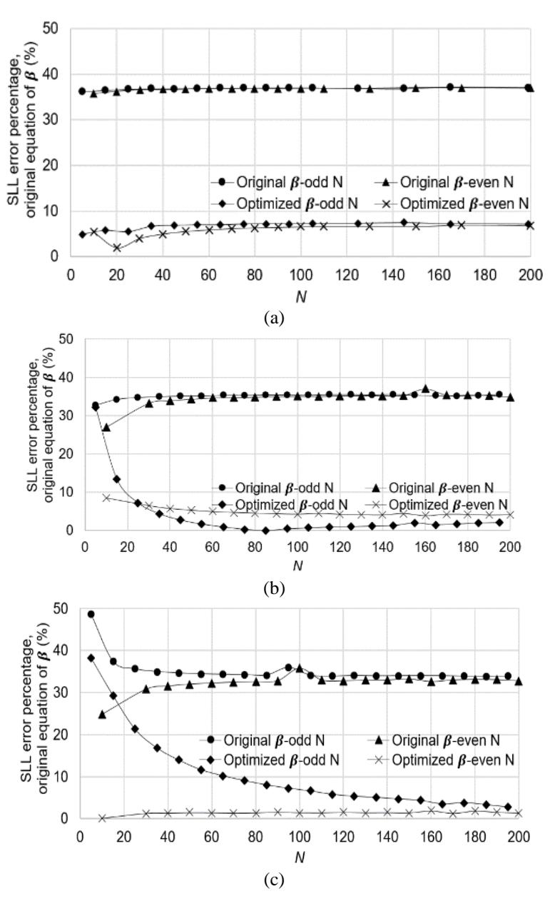
Figure 7 SLL error percentage of the obtained and targeted SLL, using original and optimized β values based on the Kaiser function for 5 ≤ N ≤ 200, (a) Targeted SLL: 25 dB, (b) targeted SLL: 35 dB, (c) targeted SLL: 45 dB.
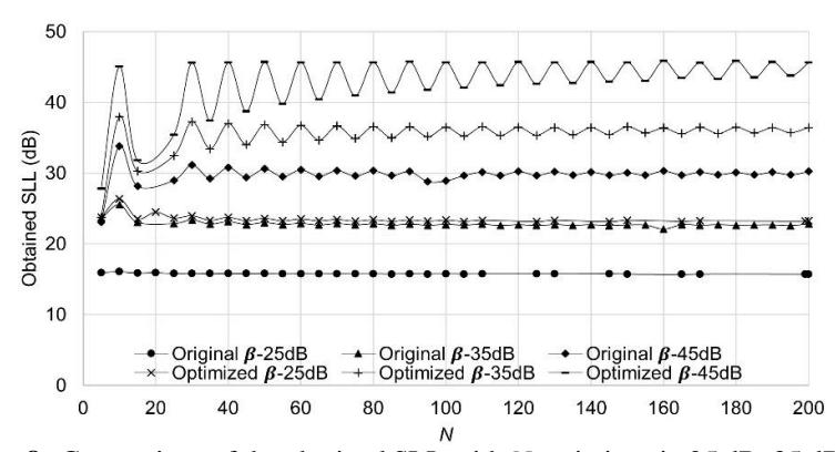
Figure 8 Comparison of the obtained SLL with N variations in 25 dB, 35 dB, and 45 dB and the targeted SLL with β values from the original and the optimized equation of β.
7 Conclusion
The potentiality of applying a Kaiser function in power-weighted antenna arrays was investigated. For specific arrangements and requirements, using a Kaiser function is a promising method for power-weighted linear antenna array designs. It was shown that the WML of the Kaiser function was broader compared to that of the Chebyshev function. In relation to the targeted SLL, the Kaiser function also demonstrated similar flexibility as the Chebyshev function. The investigation of β showed the necessity of β optimization. It was proven that the optimized β value provide a low SLL error percentage for 5 ≤ N ≤ 200. Further research is necessary to validate the optimized β values in simulation and measurement.
Acknowledgements/Funding
This research work was partially supported by the Indonesia Endowment Fund for Education (Lembaga Pengelola Dana Pendidikan, LPDP-BUDI DN) from the Ministry of Finance and the Ministry of Research, Technology and Higher Education, the Republic of Indonesia and the program of research, community services and innovation (Program Penelitian, Pengabdian kepada Masyarakat dan Inovasi, P2MI) Institut Teknologi Bandung, the Republic of Indonesia.