
1 Introduction
Universities play a crucial role in providing their students with a high-quality education. Most students attend college with the hope of laying the foundation for their future, which involves acquiring skills that will help them achieve a fulfilling career [1]. Therefore, education institutions have a responsibility to understand the path students take to complete the degree they are pursuing and to assist them in achieving their educational goals. Universities must monitor student progress and identify key components of student performance in order for them to graduate and move on to the next level.
A problem that often arises is that the process experienced by students will differ for each individual and not always produce the desired results [2]. Undesired
results can occur due to various factors,such as lack of academic monitoring from the institution or students who lack the motivation to attend classes. This will naturally have a negative impact on both parties. Graduation is one aspect of assessment in the accreditation process of a higher education institution [3]. Therefore, facing students who lack the motivation to attend classes will affect the quality of the accreditation of the educational institution. However, if there is a lack of academic monitoring, this will also make it difficult for students to graduate on time. The Faculty of Computer Science at Brawijaya University's 2020-2024 Education Guidelines state that a student can be considered to have completed their studies in a program when they have collected a minimum of 144 credit points with a minimum cumulative GPA of 2.00 and have completed other requirements [4]. This needs to be completed by the student within a maximum of 4 years of study to be classified as on-time graduation. Therefore, predicting student graduation is an essential consideration for educational institutions, in this particular case the Faculty of Computer Science at Brawijaya University, to monitor and improve or maintain the students' performance during their study period.
The previous research conducted by Ali, et al. [5] implemented a deep learning technique and obtained an accuracy rate of 72.84%. The study conducted by Rismayati, et al. [6] compared several algorithms, i.e., logistic regression, Gaussian, decision tree (DT), random forest, KNN, support vector machine (SVM), multi-layer perceptron (MLP), and adaptive boosting (AdaBoost), and then implemented the ensemble method. The multi-layer perceptron (MLP) algorithm had the best accuracy at 91.8%. Another study that used data mining techniques for classification is the research by Syahputra, et al. [7]. Based on student data attributes such as GPA, credit points, total credit points, and semester, classification was performed achieving a classification accuracy value for the Customer Relationship Management course and the Wireless Network course of 85.88% and 44.92%, respectively.
From previous research, the use of data mining methods, particularly deep learning or deep neural network algorithms, has resulted in a wide range of accuracy rates, with some being low and others performing better. There were shortcomings in the previous study by Rismayati, et al. [6], which lacked information on the hyperparameters of the trained model and on the testing results. This information was lacking because the study only focused on comparing the accuracy performance of the algorithms used to solve the problem. A weakness of another study, by Ali [5], was the use of a small amount of data, only 405 data, for the deep learning method, resulting in the model's performance not being able to be maximized in solving the same case. Thus, the accuracy of the model could still be improved.
Therefore, in this research, a deep learning method was used to predict the ontime graduation of students of the Faculty of Computer Science at Brawijaya University. The ability of deep learning to effectively extract intricate patterns from underlying data is well-known [10-13]. According to Xing & Du [11], unlike neural network and simple machine learning algorithms, deep neural networks do not require in-depth information about each attribute used. This enables the deep learning method to create a better learning model without the need for complex feature selection or preprocessing of the data. Then, due to the lack of information on the hyperparameters used in training the model with the deep learning or deep neural network algorithm, hyperparameter tuning will be performed to find the best combination of hyperparameters for predicting the ontime graduation of students. The model evaluation will be done by testing the test data based on the confusion matrix and measuring the accuracy, precision, and recall values, and comparing them with those from other methods, i.e., logistic regression and SVM.
Based on the arguments above, the challenge of this research was to perform and measure the accuracy of on-time graduation prediction of students using deep learning, which has not yet been implemented previously to classify similar graduation cases using individual academic result attributes. As its contribution, the purpose of this research was to understand whether the deep learning method is more accurate and efficient in predicting on-time student graduation than other classification methods like SVM and decision tree. As a result, educational institutions will be able to better understand the conditions of their students so they can take steps to maximize their on-time graduation.
2 Related Work
Data Mining and Deep Learning. Commonly used are data mining techniques combined with classification. The models most commonly used by previous researchers are decision tree, naïve Bayes, and SVM [12]. Some research also compared traditional methods with MLP [8, 13].
Academic Performance Prediction. Of all the prediction tasks in the educational field, academic performance prediction is the one that is studied the most. Other research established that there is a correlation between student GPA and other variables, such as heterogeneous student behavior and any social influence that can affect the students' GPA results [14-17]. However, the present research only focused on Semester GPA, which is a score on a four-point scale to quantitatively describe the academic performance of students in one semester and the course credits that students have to earn in one semester to predict academic performance related to student graduation.
Therefore, in this study, a deep learning method was used to classify whether students of the Faculty of Computer Science at Brawijaya University will be able to graduate on time. Deep neural networks do not require in-depth information about each attribute used, enabling the DNN to create a better learning model. In this study, the attributes used focus on Semester GPA and course credits for each semester. These factors were chosen because Semester GPA and course credits are the most important factors that affect student graduation time. Moreover, hyperparameter tuning was also implemented to find the best combination of hyperparameters to enhance the classification model for predicting on-time graduation of students.
3 Student Prediction Model
3.1 Data Collection
The data collection process was conducted by collecting academic data of students of the Faculty of Computer Science at Universitas Brawijaya. The obtained data consisted of academic data of the students. The data were divided based on year and semester, resulting in twelve files, covering academic data of students in the odd semesters of 2015 up to the even semesters of 2020. In each file, there were data of students with attributes, i.e., the level of study, major, cohort, student identification number, name, year, semester, short-semester status, credit-weighted average grade, credit load, credit-weighted average cumulative grade, total credits completed, average grade upon graduation, total credits completed upon graduation, and total credits required for graduation.
Each file contained 4,300 to 4,500 student data with a total of about 53,384 lines of data with 16 features. As this research focused only on students from the cohorts of 2015, 2016, and 2017, data on the students from other years were removed. The reason was that the student cohorts from 2015 to 2017 were expected to have graduated by 2022. Meanwhile, the data from student cohorts after 2017 mostly had not yet graduated. As a result, the data for the student cohorts after 2017 could not be used as real cases of graduated students. Additionally, other attributes such as credit load, credit-weighted average cumulative grade, and total credits required for graduation were not used because they are correlated with the attributes used, i.e., average grade upon graduation and total credits completed per semester upon graduation, so they were not necessary.
The average grade upon graduation (Semester GPA), also known as Indeks Prestasi (IP), is an achievement record of the learning process in university that students receive at the end of each semester. Meanwhile, course credits (in Indonesian: satuan kredit semester – SKS) express the study load of a course in a university. Students have to earn a minimum number of course credits during one semester to successfully complete it. Thus, this research used attributes such as Semester GPA from the first semester to the sixth semester, and course credits from the first semester to the sixth semester with data from 2,184 students with 12 attributes. Next, this data underwent preprocessing.
3.2 Data Preprocessing
Preprocessing must be applied on the data to improve the efficiency of processing these data [18]. The preprocessing method employed consisted of several stages. The first stage was that the researcher carried out filtering to obtain data that could be considered valid and suitable for the needs of the research. Then, data cleansing was performed to eliminate empty data. Since the class distribution of the data was imbalanced, i.e., 46.4% of students graduated after more than four years and 53.6% of students graduated within four years, resampling was carried out so that the data distribution was balanced between both classes.
There are various methods for addressing class imbalance in data, but they are generally categorized into three categories: data-level, algorithmic-level, and cost-sensitive [19]. The method used in this research falls under the data-level category. In the data-level approach, the class imbalance problem is solved by resampling, which involves modifying the amount of data by adding or removing data to achieve a balanced class distribution. The resampling method used was undersampling of the majority class, which involved creating a subset of the original data by removing a sample of the majority class. However, before that, the data was separated into training data and test data. This was done beforehand, because the test data used cannot be sampling data.
The process was then continued by eliminating outliers. In this research, data considered as outliers were those with IP (GPA) or SKS (course credits) values of 0. As a result, some data in the lower quantile were removed. This was done so that the class distribution values were more evenly distributed but not too much data was lost. Next was normalization using the min-max normalization method. Min-max normalization is a technique that involves linear transformation of the original data in order to create balanced value comparisons between the data before and after the process [20,21]. The data normalization calculation for minmax normalization can be seen in Eq. (1):
\[X_n = \frac{X_0 - X_{min}}{X_{max} - X_{min}} \tag{1}\] where \(X_n\) is the new value after normalization, \(X_0\) is the value to be normalized, \(X_{max}\) is the maximum value of the data, and \(X_{min}\) is the minimum value of the data.
3.3 Deep Learning Model
The implementation of the method in this research using deep learning was carried out in several stages, as shown in Figure 1.
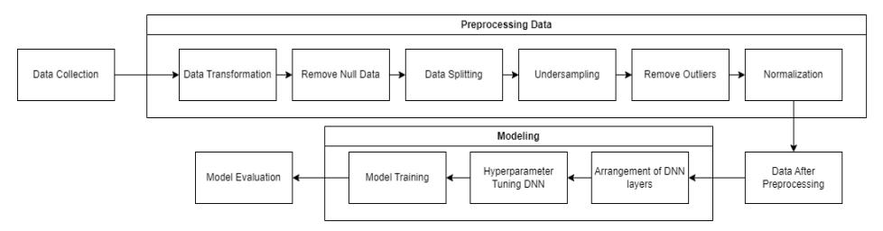
Figure 1 Implementation stages.
After the data preprocessing was completed and the data was divided into training data and validation data, the next stage was model development. Model development consists of composing the layers of the deep learning network, configuring the hyperparameters, and training and validating the model. Deep learning is a machine learning concept based on artificial neural networks [22]. The use of deep learning involves the addition of one or more hidden layers. The deep learning architecture is displayed in Figure 2.
Figure 2 Deep learning architecture.
According to Figure 2, the deep learning method is divided into three parts, i.e., an input layer, a hidden layer, and an output layer. The input layer has twelve features as the initial input attributes, consisting of the Semester GPA values for semesters 1 to 6 and the number of credit units for semesters 1 to 6. Then, in the hidden layer, the layers used included:
1. Fully Connected Layer
The linear layer, or fully connected layer, is the main layer of almost all neural network models currently in use, with a composition of linear layers and nonlinear modules such as the sigmoid and ReLU layers [23]. The fully connected layer is an implementation layer of MLP that serves to recognize important features that influence the process of training the model and therefore the resulting prediction. The function of the fully connected layer is expressed in Eq. (2):
\[y = xA^T + b (2)\] where denotes the layer input value, are the inverse weights, and is the bias.
2. Activation Function
The activation function serves to change the artificial neural network model into a non-linear function and increase the capabilities of the artificial neural network even further. If an artificial neural network does not use an activation function, then the output signal (output) will only be a simple linear function that is only a polynomial of degree one, commonly called a single-layer perceptron [24]. In the classification process, the Rectified Linear Unit (ReLU) in the hidden layer and the sigmoid activation function were used in this research.
The ReLU activation function is a function used to apply a better linear function. ReLU works with a threshold value of 0, so ReLU will produce 0 when < 0, and conversely, ReLU will produce a linear function when ≥ 0 [25]. ReLU is more efficient than other activation functions because it only activates a few neurons at a time [24]. The equation for the ReLU activation function is written in Eq. (3):
\[ReLU(x) = (x)^{+} = max(0, x)\] (3)
where x is the activation function input and () + is the activation function output.
Currently, there are many activation functions in use, and one of them is the sigmoid (logistic function) activation function used in the output layer of the neural network for classification [26]. The sigmoid activation function is a suitable choice for binary classification cases with normalization between 0 and 1. The sigmoid function is also not symmetrical with respect to the value 0, which means that the signs of all neuron output values will be the same, but this problem can be corrected by scaling the sigmoid function [24]. The equation for the sigmoid activation function is written in Eq. (4):
\[Sigmoid(x) = \sigma(x) = \frac{1}{1 + e^{-x}} \tag{4}\] where is the activation function input and () is the activation function output.
3. Batch Normalization Layer
The batch normalization greatly reduces the training time by normalizing not only the input layer but also the input for the other layers in the network [27]. The function of the batch normalization layer is expressed in Eq. (5):
\[y = \frac{x - E[x]}{\sqrt{Var[x] + \epsilon}} * \gamma + \beta \tag{5}\] where denotes the activation function input, is epsilon, is the weight, and is the bias value.
3.4 Experiment
In the testing and analysis stage, the model underwent hyperparameter tuning with the help of the Optuna Library by Akiba, et al. [28]. Optuna is a Python library that functions to automatically tune hyperparameters. The hyperparameter search process in Optuna in this research used a sampling method called the Tree-Structured Parzen Estimator (TPESampler). The following is the design of the hyperparameter tuning test on the DNN model.
Table 1 Hyperparameter Tuning test for DNN.
| Hyperparameter | Value | ||
|---|---|---|---|
| Optimizer | Adam | SGD | RMSprop |
| Learning Rate | 0.00001 – 0.1 | ||
| Dropout | 0 – 0.5 | ||
| Number of Nodes | 16 – 128 | ||
| Epoch | 200 – 250 | ||
| Number of Combination Layers | 3 – 5 |
Next wasthe design of the hyperparameter tuning test for the comparison method. The methods used for comparison were logistic regression and SVM. The following table is the hyperparameter tuning test for the comparison method.
Table 2 Hyperparameter tuning test for comparison method.
| Hyperparameter | Value | ||
|---|---|---|---|
| 𝐶 | 10-7 - 107 | ||
3.5 Evaluation Metrics
After obtaining the best combination of hyperparameters, an evaluation was conducted using the confusion matrix to determine the values of accuracy, precision, and recall, as well as an analysis to understand the influence of each hyperparameter on the test results.
4 Experimental Results and Discussion
This section is divided into two main parts. The first part describes an exploration of the hyperparameter results and the second part is the discussion of the results obtained.
4.1 DNN Hyperparameter Tuning
The hyperparameters that were tested were the optimizer, learning rate, dropout, number of nodes, maximum epoch, and number of combination layers. In this test, hyperparameter tuning was conducted with the help of the Optuna library using the TPESampler method. The results of the hyperparameter tuning test can be seen in Table 3. From the results, Optuna can also visualize the sequence of the most influential hyperparameters on the accuracy of the validation data as shown in Figure 3.
Accuracy Dropout 0 … Optimizer State 0.8152 0.3660 … SGD COMPLETE 0.4988 0.1521 … RMSprop COMPLETE 0.7436 0.2962 … Adam COMPLETE 0.4988 0.0610 … Adam COMPLETE 0.8037 0.0442 … SGD COMPLETE … … … … … 0.4988 0.2581 … RMSprop PRUNED 0.8222 0.2919 … SGD PRUNED 0.7436 0.3125 … SGD COMPLETE
Table 3 Hyperparameter tuning results for DNN.
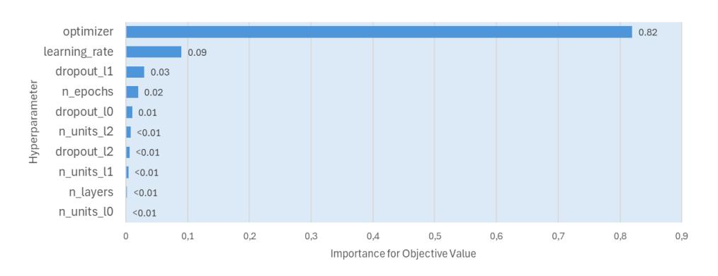
Figure 3 Hyperparameter importance DNN.
Based on Figure 3, the optimizer was the hyperparameter that played the most influential role in increasing the accuracy of the validation with an influence of 82% and a learning rate of 9%.
4.2 DNN Model with Best Hyperparameter
After conducting hyperparameter tuning on the DNN with the help of the Optuna library, the next step was to test the best hyperparameters. The purpose of this test was to determine the effect of hyperparameter tuning on the accuracy level of the proposed on-time graduation prediction system for students. The best hyperparameter test values occurred in trial 33, which achieved an accuracy of 86.61% with the following hyperparameter values: number of combination layers (Linear, ReLU, BatchNorm, Dropout) = 4, number of nodes in the first layer = 118 with dropout value 0.3393, number of nodes in the second layer = 83 with dropout value 0.0349, number of nodes in the third layer = 88 with dropout value 0.0491, number of nodes in the fourth = 65 with dropout value 0.4169, the epoch = 244, the learning rate = 0.0710. The optimizer used was SGD. Figure 4 displays the accuracy and loss plot of the DNN model test with the best parameters, and Figure 5 shows the confusion matrix results obtained from the test with the best parameters.
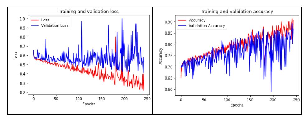
Figure 4 Accuracy and loss plots with the best hyperparameter DNN.
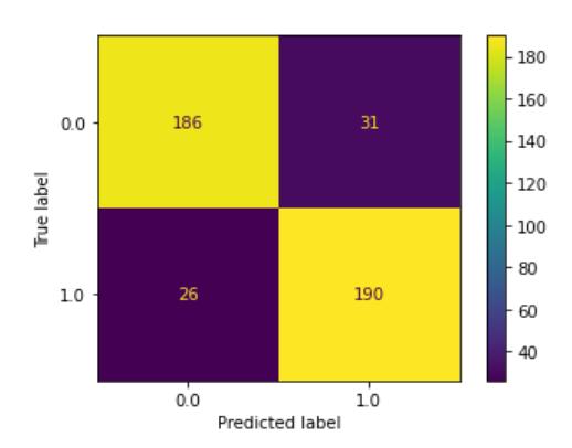
Figure 5 Confusion matrix with the best hyperparameter DNN.
Based on Figure 4, it can be observed that the model gradually reached higher accuracy and lower loss as the number of epochs increased. This indicates that the training process of the model proceeded effectively. However, through the change in loss values, it can be inferred that the model experienced overfitting. Next, the results of the confusion matrix are displayed in Figure 5. In Figure 5, label 0.0 denotes 'failing to graduate on time' and label 1.0 denotes 'graduating on time'. In Figure 5, it is also possible to see the values of accuracy, precision, recall, and F-measure, as stated in Table 4.
Table 4 DNN model results.
| Class | Precision | Recall | F1-score | Accuracy | |
|---|---|---|---|---|---|
| Graduate On Time | 0.88 | 0.86 | 0.87 | ||
| Not Graduate On Time | 0.86 | 0.88 | 0.87 | 0.87 | |
Based on Table 4, it can be seen that the model achieved a precision of 0.88, recall of 0.86, and F1-score of 0.87 for class 1 (graduating on time), and a precision of 0.86, recall of 0.88, and F1-score of 0.87 for class 0 (failing to graduate on time).
4.3 Model Comparison
This section presents the results of additional testing, specifically performing hyperparameter tuning on the comparison method. The methods that were tested here were logistic regression and SVM, while the hyperparameter being tested was the value of . The results of the hyperparameter tuning test can be seen in Table 5.
Table 5 Hyperparameter tuning results for comparison methods.
| Accuracy | Classifier | 𝑪 | State |
|---|---|---|---|
| 0.7043879908 | SVC | 0.5518315614 | COMPLETE |
| 0.8221709007 | LogReg | 835,702.8564357880 | COMPLETE |
| 0.5011547344 | SVC | 0.0000025954 | COMPLETE |
| 0.7020785219 | SVC | 3.0124504179 | COMPLETE |
| 0.5011547344 | SVC | 0.0025025813 | COMPLETE |
| … | … | … | … |
| 0.7759815242 | LogReg | 143,333.9467249480 | COMPLETE |
| 0.7667436490 | LogReg | 28,738.8087576687 | COMPLETE |
| 0.7736720554 | LogReg | 80,512.6356558365 | COMPLETE |
From this process, the best hyperparameters were obtained using the logistic regression algorithm and a value of of 796,696.077. Using this hyperparameter value, the model achieved an accuracy rate of 82.67%. Table 6 explains the results of the confusion matrix obtained in the test with the best parameters. Next, the confusion matrix results for the comparison method with the best hyperparameter are displayed in Figure 6.
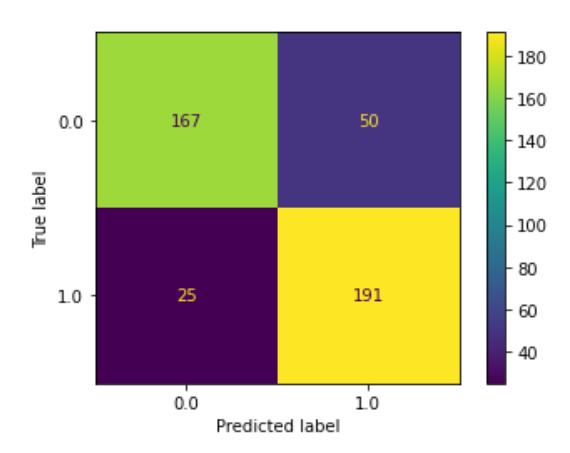
Figure 6 Confusion matrix with the best comparison method.
Table 6 Best Comparison Method Results
| Class | Precision | Recall | F1-score | Accuracy | |
|---|---|---|---|---|---|
| Graduate On Time | 0.79 | 0.88 | 0.84 | ||
| Not Graduate On Time | 0.87 | 0.77 | 0.82 | 0.83 | |
Based on Table 6.4, it can be seen that logistic regression achieved a precision of 0.79, recall of 0.88, and F1-score of 0.84 for class 1 (graduating on time), and a precision of 0.87, recall of 0.77, and F1-score of 0.82 for class 0 (failing to graduate on time). Therefore, with the best hyperparameter for each method, the comparison of accuracy is shown in Figure 7.
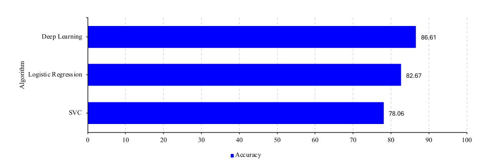
Figure 7 Accuracy comparison between methods.
4.4 Discussion
4.4.1 Hyperparameter Tunning Test for DNN Analysis
The results of the DNN model's hyperparameter tuning process using Optuna (see Figure 3) show that the optimizer and learning rate are the hyperparameters that have a significant effect on the model's accuracy, followed by other hyperparameters such as the number of epochs.
The optimizer in DNN is a method that determines how the weights are changed in the DNN model with the gradient values obtained from the training process. As shown in Figure 7, the optimizer is a hyperparameter that has a significant influence on increasing the accuracy because the weight update method for each optimizer is different. Therefore, the use of a suitable optimizer is required. In the testing of the optimizers, the optimizers determined were Adam, SGD, and RMSprop. With Optuna, which uses TPESampler or the Tree-Structured Parzen Estimated Approach, found that the optimizer with the best result obtained was SGD with an accuracy value of 86.61%.
The learning rate in DNN is a value that serves to determine the change in weight values with the gradient values in the training process. The learning rate value ranges from 0 to 1. If the learning rate value is larger or closer to 1, it means that the weight value change will also be faster. Nonetheless, the accuracy of each network will decrease, while if the learning rate value is smaller or closer to 0, it means that the weight value change will also be slower. However, the accuracy of each network will also increase. In the testing of the learning rate, the values determined ranged from 0.00001 to 0.1. The learning rate value with the best result obtained was 0.0710 with the SGD optimizer, which achieved an accuracy value of 86.61%. With the same optimizer, the learning rate values with the worst results were 0.0450 and 0.0005, with accuracy values of 66.05% and 70.2%, respectively.
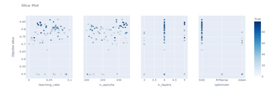
Figure 8 Hyperparameter search distribution in DNN.
Based on the distribution and spread of the hyperparameter search values in Figure 8, the optimizer greatly influences the result of the model training. The RMSprop and Adam optimizers were unable to learn the relationships between the data in the present case of predicting on-time graduation or were indicated to be experiencing underfitting, resulting in poor accuracy. Meanwhile, the SGD optimizer produced better accuracy and the training process proceeded well. This is what causes Optuna to focus the search for the optimizer hyperparameter on the SGD optimizer, resulting in the best accuracy with a value of 86.61%. Based on the testing of the optimizer hyperparameter, it can be concluded that the most optimal optimizer in the case of predicting on-time graduation for students is the SGD optimizer.
Based on the distribution and spread of the hyperparameter search values in Figure 8, the most optimal hyperparameter learning rate ranged from 0.05 to 0.075. For learning rate values above 0.075, the best accuracy obtained was only around 80% to 82%, while if the learning rate value was below 0.05, the best accuracy obtained was only around 83% to 85%. The learning rate value influences the calculation of the change in weight values, so the smaller the learning rate value, the slower the change in weight values, while the larger the learning rate value, the faster the change in weight values. Therefore, it can be concluded that the learning rate value cannot be too large or too small and requires the search for an optimal learning rate value and there is no certain learning rate value. In addition, this hyperparameter learning rate also depends on the selection of the appropriate optimizer hyperparameter. Therefore, with the same range of learning rate values but using different optimizers, a significant difference in accuracy can occur.
4.4.2 DNN Model with the Best Hyperparameters Test Analysis
Based on the accuracy and loss plot in Figure 4, it can be seen that the model's accuracy is increasing, and the loss is decreasing. This proves that the model's training process is proceeding well. In the testing process, it can be seen that the movement of the accuracy value is also increasing, but there is an oddity in the movement of the loss.
The lowest loss in the testing process occurred around epoch 120 and from then on it began to move unstably. This resulted in the model being indicated to be experiencing overfitting, which means the model is indicated to not be able to work well on new data that it has not seen before. In Figure 5, the confusion matrix of the model after testing on the test data is displayed. Based on the values of precision and recall obtained, it can be seen that the model does not have special treatment for a certain class, which means that the DNN model can classify both class 1.0 (graduating on time) and class 0.0 (failing to graduate on time) well and there are no signs of overfitting. The following is a comparison of the class labels and the model's prediction results.
| IP_1 | SKS_1 | IP_2 | SKS_2 | IP_3 | … | IP_6 | SKS_6 | LABEL | PREDICTION |
|---|---|---|---|---|---|---|---|---|---|
| 3.81 | 19 | 3.45 | 19 | 3.76 | … | 3.94 | 24 | 1 | 1 |
| 3.10 | 19 | 3.39 | 19 | 3.69 | … | 3.93 | 23 | 1 | 1 |
| 3.08 | 19 | 3.10 | 19 | 3.23 | … | 3.54 | 23 | 0 | 1 |
| 3.84 | 19 | 3.75 | 20 | 3.81 | … | 3.35 | 23 | 1 | 0 |
| 3.74 | 19 | 3.24 | 19 | 3.83 | … | 3.00 | 18 | 0 | 0 |
Table 7 Comparison of actual data labels with predicted results.
In Table 7, the comparison of the model's prediction with the supposed class label is shown, followed by the attributes of each data from the top-5 test data. Based on Table 7, it is quite difficult to see how the model can make a prediction of 1 (graduating on time) or 0 (failing to graduate on time) because the attribute values are relatively varied. However, through the model's prediction errors in data 3 and 4, it can be understood that the attribute that significantly affects the prediction based on Table 7 is the attribute IP_6, or the IP (GPA), in the sixth semester. The prediction error occurred because when the student's IP (GPA) in the sixth semester is above 3.5, the model is more likely to predict the data as a student who will pass on time, or class 1. On the other hand, if the student's IP (GPA) in semester 6 is below 3.5, the model is more likely to predict the data as a student who will fail to graduate on time, or class 0. Therefore, a prediction error occurred in data 3, where the model predicted that the student would graduate on time because the student's IP (GPA) in semester 6 was above 3.5, but the actual label of the data was failing to graduate on time. The same goes for the prediction error in data 4, where the model predicted that the student would fail to graduate on time because the student's IP (GPA) in semester 6 was below 3.5, but the actual label of the data was graduating on time.
4.4.3 Comparison Method Analysis
A comparative test was conducted by searching for hyperparameters using Optuna. The methods to be used as a comparison were SVM and logistic regression. The hyperparameter to be searched for was the value of . The value of in SVM, also known as the cost, is a regularization hyperparameter that optimizes the SVC model to prevent errors in data classification. The value of must be a positive value. When the value of is too large, the SVM algorithm will try to minimize classification errors as much as possible. This will eliminate the generalization property of the classification algorithm, causing the decision boundary, or regularization boundary, to become very small. When the value of is too small, the SVM algorithm will try to minimize classification errors as much as possible. This is because the smaller the value of , the larger the regularization boundary or decision boundary applied to the training process, resulting in a higher proportion of errors occurring in the classification process. The same is true for the application of the value of in the logistic regression method. Therefore, the value of cannot be too large or too small and it is necessary to find the optimal value of .
Based on the results of the testing, the best value of obtained was 796,696.0771973614 with an accuracy of 82.67%, using the logistic regression method. Meanwhile, the worst value of obtained was 0.0001463588402424 with an accuracy of 50.11% using the logistic regression method. Therefore, based on the search for hyperparameters in the comparison method in Table 5, the optimal value of to be used in this case ranged from 10,000 to 100,000 with the best value of being 796,696.0771973614. It can be concluded that the value of C cannot be too large or too small, so it is necessary to search for the optimal value of , and the value of also does not have a specific value.
According to the accuracy comparison graph in Figure 7, it is known that deep learning had the highest accuracy at 86.61%, followed by logistic regression with an accuracy of 82.67%, and SVM with an accuracy of 78.06%. The results obtained in this research were roughly the same as those obtained by Rismayati, et al. [6], where the multi-layer perceptron (MLP) or deep learning method had the best accuracy, followed by simple algorithms such as logistic regression and SVM. This is because deep learning is a better method when the data available is sufficient. Unlike logistic regression and SVC, which are linear models, deep learning uses many combinations of hidden layers, causing many non-linear transformations to occur in the data training process, allowing for good classification of more complex data. Basic machine learning algorithms such as SVM and logistic regression also require more explicit preprocessing so that the data is easier to understand and the classification results are better. This is what makes SVM and logistic regression better in cases where the amount of data is smaller and the data is not too complex. The following shows the correlation of each feature used in this case of predicting on-time graduation in Figure 9.
Based on Figure 9, it can be seen that the relationship between the features used for classification, such as the IP (GPA) and SKS (course credits) features and the class feature LULUS_TEPAT_WAKTU tends to be weak with the best correlation value of 0.39 with the IP_6 feature. This is another reason why the logistic regression and SVM methods do not perform better than the deep learning method. With the weak correlation value of the classification features with the class feature, it makes the data more complex and more difficult to classify. Therefore, with complex data conditions, a sufficient amount of data, the same preprocessing method, and the hyperparameter search process, the deep learning method is the best method. Therefore, in this study it was concluded that, with the same preprocessing method and hyperparameter search process, the deep
learning method was the best method in solving the case of predicting on-time graduation of students of the Computer Science Faculty of Universitas Brawijaya.
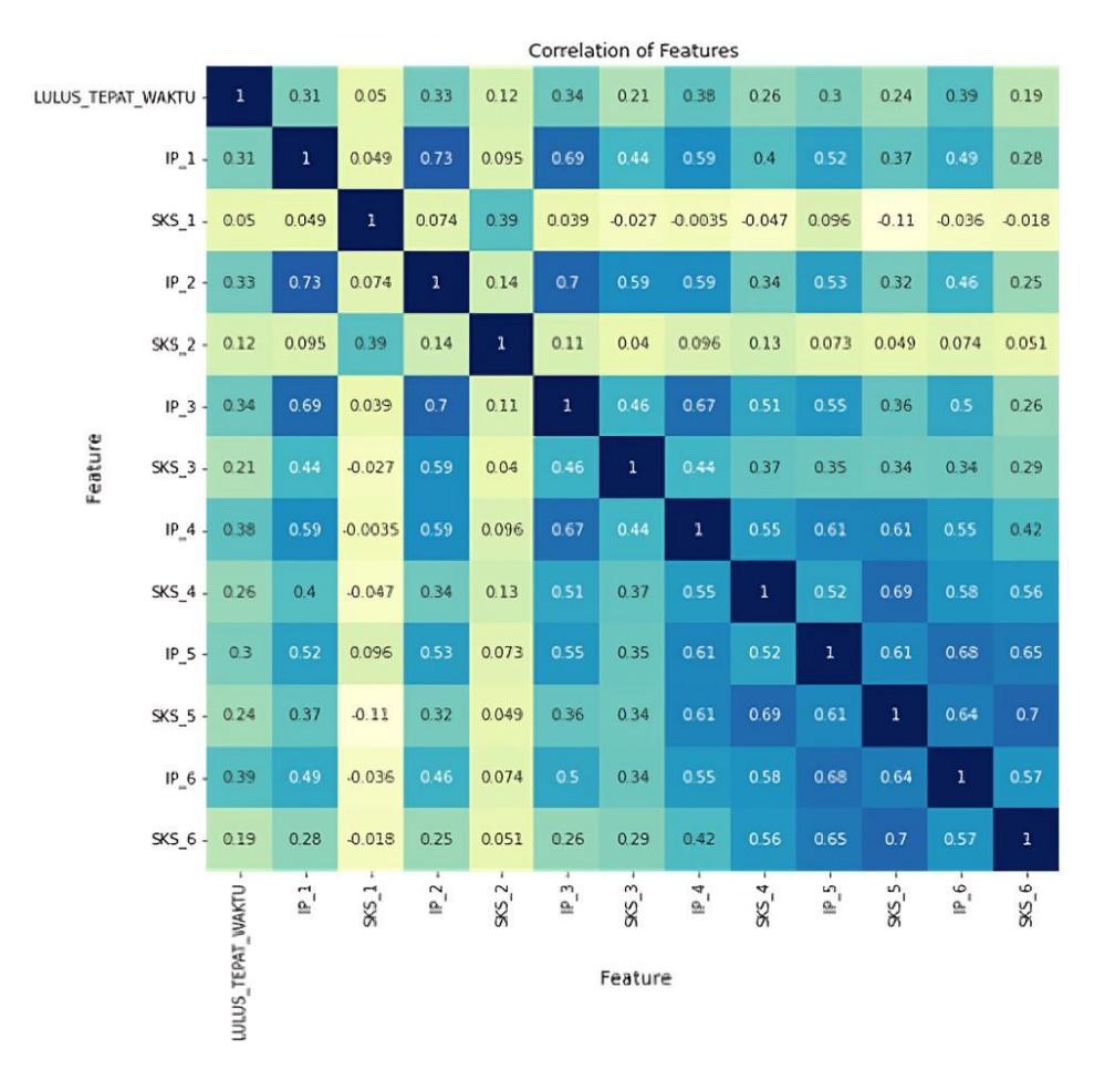
Figure 9 Feature correlation.
5 Conclusion
Based on the implementation and testing conducted on on-time graduation prediction of students using the deep learning method, it can be concluded that in the hyperparameter tuning test using Optuna, a combination of hyperparameters was obtained consisting of a combination of four layers (which on every layer consist of Linear, ReLU, BatchNorm, Dropout), number of nodes in the first layer = 118 with a dropout value of 0.3393, number of nodes in the second layer = 83 with a dropout value of 0.0349, number of nodes in the third layer = 88 with a dropout value of 0.0491, number of nodes in the fourth layer = 65 with a dropout
value of 0.4169, 244 epochs, a learning rate of 0.0710, and the SGD optimizer. The hyperparameter tuning process resulted in a model with an accuracy of 86.61% on the test data. In the test with the comparison methods of logistic regression and SVM, the best result was obtained with an accuracy of 82.67% using the logistic regression method, and a value of equal to 796,696.0771973614. Therefore, it can be concluded that the deep learning method was the best and most optimal method for solving the case of on-time graduation prediction of students.
However, there were still some shortcomings of this study that can be addressed by adding more data (actual data without the use of resampling) to reduce the indication of overfitting in the deep learning model. Further, it is hoped that other hyperparameter tuning methods such as grid search can be implemented to test and evaluate the model with every combination specified in the hope of finding a more accurate combination of hyperparameters to achieve an even higher accuracy value and provide a detailed comparison between hyperparameters.