
1 Introduction
Surveillance camera networks, commonly known as CCTV (closed circuit television), were developed by German scientists in 1942 [1]. They are extensively used for various purposes, including security, safety, entertainment, and efficiency improvement [2]. Various algorithms process CCTV output for applications such as object detection, classification, and tracking [2]. In Indonesia, toll road CCTV data is publicly accessible through web or mobile applications [3]. This feature significantly enhances real-time monitoring of traffic conditions. Additionally, this CCTV data is used in various intelligent transportation system (ITS) applications [4], such as vehicle counting, automatic number plate recognition (ANPR), and incident detection [5].
Vision-based sensors can classify vehicles based on geometry, appearance, texture, and a mixed approach [6]. Depending on the speed and camera perspective, these applications can be deployed in both urban and highway settings. One popular implementation of CCTV data on toll roads is automatic vehicle classification (AVC), which classifies vehicles based on type. Vehicle type recognition (VTR) aims to categorize vehicles into high-level classes such as buses, sedans, vans, trucks, etc. [6]. Many traffic studies and analyses utilize automated VTR systems. Additionally, one study has been conducted to determine electronic toll rates using this VTR system [7].
Annotation tools are essential for creating labeled datasets with the vast amounts of available data for effective machine-learning models [8]. AVC and VTR systems rely on these tools to classify vehicles accurately. To achieve high performance, deep learning models require large-scale datasets with precise annotations. However, manual annotation is time-consuming, tedious, and costly [9], prompting the need for automatic or semi-automatic annotation methods [10].
This paper proposes an end-to-end pipeline called saLFIA (semi-automatic Live Feeds Image Annotation) to create annotated datasets from public CCTV images. The pipeline includes retrieving images, preprocessing them, and auto-labeling them into vehicle categories based on Indonesian toll road fare classifications. The saLFIA tool generates numerous annotated images using flexible HTTP resources and allows for manual correction to improve annotation quality. This approach simplifies annotation and enhances efficiency, presenting a new method for creating annotated datasets in a single operation.
This paper is organized as follows. Section 2 describes related studies on annotation tools for vehicle classification. Section 3 describes the saLFIA tool, including the saLFIA pipeline, function module, pre-trained model, and implementation of an Indonesia CCTV case study. The conclusion and future work are presented in the last section.
2 Related Works
Many studies provide open datasets for AVC that classify vehicle classes according to their respective research topics [11-14]. Various image annotation tools have been developed to simplify and speed up the annotation process. These tools are essential for producing high-quality ground truth (GT) from large-scale visual datasets. Annotation tools can be manual or semi-automatic. Some widely used manual annotation tools available for open access include LabelImg [15], LabelMe [16], and imglab [17]. While manual annotation tools offer high accuracy, they are time-consuming. The manual annotation tool is a web-based and desktop interface. These tools provide polygons, rectangles, circles, lines, or points as object boundaries and save the annotation results in formats such as XML, Pascal VOC, COCO, and YOLO.
Semi-automatic annotation tools are designed to enhance the speed of the annotation process using models to generate annotations across multiple images. Examples of these tools include LOST [18], iVAT [19], COCO Annotator [20], and CVAT [21]. LOST [18] operates in two stages: single-stage and two-stage annotation. The single-stage annotation uses the Single Image Annotation (SIA) process to manually create baseline bounding box annotations. The two-stage annotation combines SIA with Multi Image Annotation (MIA), which finds visual similarities within a cluster to assign class labels. iVAT [19] is a video annotation tool that employs linear interpolation and template-matching algorithms for semi-automatic and automatic annotation, working within an interactive and incremental learning framework. COCO Annotator [20], a webbased tool, offers image segmentation, object instance tracking, and object labeling. It provides semi-automatic annotation using methods like the Magic Wand for similar pixel color and shade selection and a semi-trained model like MaskRCNN for annotation. CVAT [21] is an interactive video and image annotation tool for computer vision that supports multiple annotation formats. It supports automatic labeling with several algorithms, such as Faster-RCNN, Mask-RCNN, RetinaNet, YOLOv3, and YOLOv7.
Table 1 provides a comparative overview of features across various recent annotation tools. Several annotation tools utilize deep learning models for object detection tasks, which can be categorized into two-stage and one-stage methods.
| Tools | Input | Method | Platform | Output Format | |
|---|---|---|---|---|---|
| LabelImg [15] | Image | Manual | Desktop-based | YOLO, Pascal VOC | |
| LabelMe [16] | Image | Manual | Web-based | JSON | |
| ImgLab [17] | Imaga | Manual | Desktop-based, | Dlib XML, Dlib pts, | |
| Image | wanuar | Web-based | Pascal VOC, COCO | ||
| LOST [18] | Image | Cluster image similarity | Web-based | CSV | |
| iVAT [19] | Video/ | Linear Interpolation, | Desktop-based | Video Annotation | |
| images | Template Matching | Desktop-based | Database | ||
| Coco Annotator [20] | Images | MaskRCNN Magic Wand, DEXTR | Web-based | COCO | |
| CVAT [21] | 37.1 | Faster-RCNN, Mask- | YOLO, Pascal VOC, | ||
| Video/ images | RCNN, RetinaNet, | Web-based | COCO, MOT, KITTI, | ||
| YOLOv3, YOLOv7, etc | CVAT, etc | ||||
| saLFIA [proposed] | Live-feed images | YOLO, SSD | Script-based | YOLO, Pascal VOC | |
Table 1 Recent annotation tools feature comparison.
Two-stage methods, such as Faster R-CNN [21] and R-FCN [22], focus on enhancing detection accuracy. On the other hand, the one-stage method
prioritizes detection speed, as exemplified by SSD [22], RetinaNet [23], and YOLO v3 [24]. When it comes to automatic annotation programs that prioritize speed, the one-stage methods are a better fit. Studies have shown that SSD and YOLOv3 outperform other deep learning algorithms in terms of speed [25].
Consequently, the saLFIA tool utilizes pre-trained YOLOv3 and SSD models for image annotation. It processes images crawled from live stream URLs, extracting and annotating data. The resulting annotations consist of rectangular bounding box coordinates with label classes stored in YOLO or Pascal VOC format. This tool operates via a command line interface.
3 saLFIA
3.1 saLFIA Pipeline
The saLFIA tool comprises three main functions: image crawling, object detection, and annotation, as depicted in Figure 1. Image crawling is responsible for gathering images from a specified source URL. The user begins by defining the URL for the live feed and setting the number of images they wish to capture. This function automates the process of collecting images from the defined source. The second function is object detection, which involves detecting objects within the collected images using a chosen model, such as YOLO or SSD. The user configures the object detection model and sets the corresponding weight parameters. This step leverages the capabilities of the selected model to identify and classify objects in the images. The final function is annotation, which generates annotation files for each image processed. These annotation files and the raw images are saved in a designated location specified by the user. This function is crucial in creating a dataset in which detailed annotations accompany each image. The quality of the dataset improves with more accurate detection models, as better models reduce the need for manual corrections and enhance the overall dataset quality.
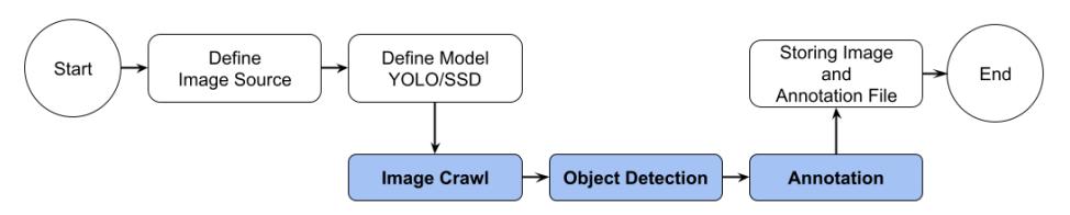
Figure 1 saLFIA scheme.
3.2 saLFIA Function Modules
3.2.1 Image Crawling
The first module of this program is an image crawling module that retrieves images from a given URL. The first step in retrieving and saving images is to initialize the number of images to be obtained (N), along with the URL and directory to store the images in a certain directory. We retrieve the picture from the URL for each image i (where i ∈{1,2,...,N}), decode the image data into a numeric array, and then save the image locally with a timestamp as the filename. Following a second reading, each image is enlarged using padding to preserve its aspect ratio and then transformed from BGR to RGB format. After being normalized and transposed, the picture is turned into a tensor to be processed further.
3.2.2 Object Detection
In the object detection phase, the processed image tensor is fed into a YOLOv3 or SSD model. As shown in Figure 2, the YOLOv3 architecture divides an image into a grid of equal size, with each grid cell predicting only one object and a bounding box along with the confidence score of the objects present in that grid. YOLO has undergone several improvements to enhance detection accuracy while maintaining high-speed performance.
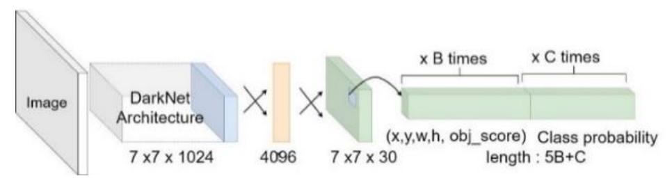
Figure 2 YOLO architecture.
Conversely, Figure 3 illustrates the SSD architecture, which consists of two main parts. In the first part, SSD extracts feature maps using the VGG16 base network. The second part applies convolutional filters on these feature maps to detect objects, with additional feature layers used to enhance the detection capabilities.
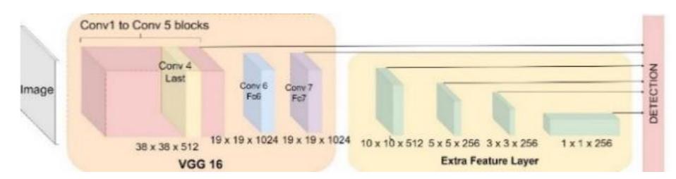
Figure 3 SSD architecture.
3.2.3 Annotation
Following object detection, the module performs annotation by applying nonmaximum suppression (NMS) to filter out overlapping bounding boxes based on confidence and intersection-over-union (IoU) thresholds. According to the parameter definitions, the class data and bounding box coordinates generated from this process are stored in either YOLO or Pascal VOC format. The results are then written to a '.txt' or '.xml' file, where bounding box coordinates are converted from absolute to normalized values. Labels for each detected object are saved alongside these coordinates, ensuring that the results are accurately recorded for further analysis or use.
3.3 Pre-trained Model
We developed a pre-trained model using several initial images for training. The distribution of objects across different classes was calculated based on the total number of initial images used for each model, as detailed in Table 2. For example, with 20 initial images, there were 77 objects in class 1, 33 in class 2, 24 in class 3, 9 in class 4, and 10 in class 5. The initial image set includes both the existing dataset and new images, resulting in data sets of 50, 100, 200, and 500 images. Each data set provides information on the number of objects present in each class.
| Total Initial Images | Class 1 | Class 2 | Class 3 | Class 4 | Class 5 |
|---|---|---|---|---|---|
| 20 | 77 | 33 | 24 | 9 | 10 |
| 50 | 228 | 91 | 48 | 20 | 24 |
| 100 | 486 | 174 | 99 | 33 | 34 |
| 200 | 980 | 357 | 204 | 54 | 60 |
| 500 | 2309 | 717 | 500 | 78 | 95 |
Table 2 Object distribution of initial images.
The model generated at this stage is named according to the algorithm and the number of initial images. For instance, SSD_20 denotes the SSD algorithm trained with 20 initial images, while YOLO_20 denotes the YOLO algorithm trained with 20 initial images. Consequently, ten pre-trained models were generated, each representing a combination of an algorithm and a specific number of initial images.
3.4 Indonesia Toll Road CCTV Case Study
In this section, we measure the effectiveness of the annotation pipeline using the YOLOv3 and SSD detection models. To evaluate saLFIA, we performed two stages of measurements: average precision for each class and manual counting of misdetection and mislabeling. The case study used CCTV live-feed data to focus on vehicle classification problems based on Indonesian toll road tariff regulations. The GT test data consists of 80 images from 4 CCTV cameras, with 20 images from each camera. Additionally, we provide the number of objects for each class from a specific camera in Table 3.
| Image Source | Images | Total Object | Class 1 | Class 2 | Class 3 | Class 4 | Class 5 |
|---|---|---|---|---|---|---|---|
| Camera-1 | 20 | 128 | 74 | 29 | 16 | 3 | 6 |
| Camera-2 | 20 | 92 | 62 | 8 | 10 | 5 | 7 |
| Camera-3 | 20 | 126 | 73 | 26 | 15 | 7 | 5 |
| Camera-4 | 20 | 34 | 7 | 6 | 13 | 3 | 5 |
| Total data | 80 | 380 | 216 | 69 | 54 | 18 | 23 |
Table 3 GT test data object composition.
In this study, vehicle classification includes five distinct classes based on the number of vehicle axles, as outlined in Figure 4, following Indonesian toll road tariff regulations. The selection of camera locations considers the visibility of the vehicle's axles and the types of vehicles frequently observed on the road. It is important to note that the data set was imbalanced: class 1 has a significantly higher number of images compared to classes 4 and 5, which correspond to vehicles with more axles.
Figure 4 Object example images for each class of vehicles.
The evaluation result of the first stage is shown in Figure 5. This experiment analyzed the effect of increasing the number of initial images on the model's accuracy. The testing results show that the mean average precision (mAP) value increased with the addition of more initial images. However, in classes 4 and 5, the mAP value decreased due to the relatively insignificant data addition compared to other classes. SSD_20 achieved an mAP value of 0.5, 0.7 for SSD_100, and a maximum mAP value of 0.850 for SSD_500. Conversely, YOLO_20 obtained an mAP value of 0.2, 0.7 for YOLO_200, and a higher maximum mAP than SSD, with 0.874 for YOLO_500.
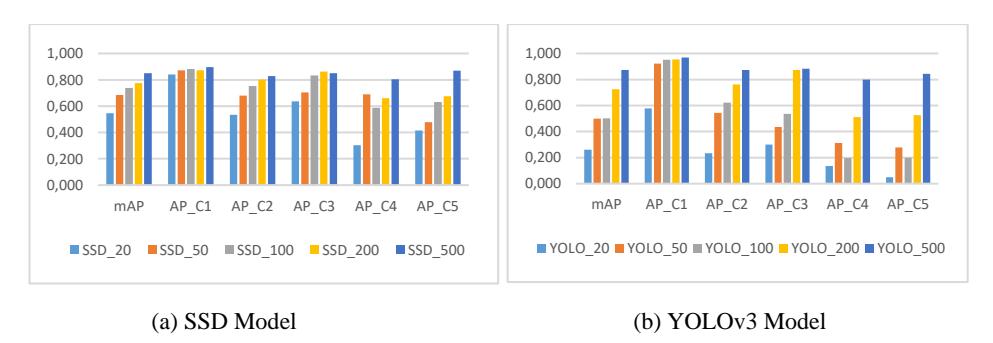
Figure 5 Evaluation results over class.
In class 1, for 20 initial images with 77 objects, SSD outperformed YOLOv3, achieving an AP value of 0.839 compared to YOLO's 0.579. For classes 2, 3, and 4, SSD with 50 initial images surpassed an AP value of over 0.65. In class 5, SSD reached an AP value over 0.65 with 200 initial images. In contrast, the YOLOv3 model achieved an AP value over 0.65 in classes 2 and 3 with 200 initial images and in classes 4 and 5 with 500 initial images.
Table 4 Misprediction evaluation results.
| Model | SSD 20 | SSD 50 | SSD 100 | SSD 200 | SSD 500 | YOLO 20 | YOLO 50 | YOLO 100 | YOLO 200 | YOLO 500 |
|---|---|---|---|---|---|---|---|---|---|---|
| Misdetection | 94 | 59 | 46 | 44 | 25 | 265 | 141 | 120 | 30 | 8 |
| Mislabeling | 156 | 101 | 80 | 76 | 45 | 267 | 148 | 134 | 65 | 28 |
The second stage results, shown in Table 4, determined the number of manual corrections made by the annotator based on the GT label. The number of corrections for SSD and YOLO decreased as the initial images increased. SSD showed low misdetection and mislabeling rates from the initial phase, with SSD_20 to SSD_50. It reached minimum misdetection and mislabeling rates of 25 and 45, respectively, with SSD_500. Meanwhile, YOLO began to show low misprediction rates starting from YOLO_200. YOLO_500 achieved impressive results with only 8 misdetections and 28 mislabelings out of 380 objects.
Figure 6 illustrates a visual comparison of model predictions across all cameras. This result demonstrates the evolving performance of the models in predicting objects, showing gradual improvement with the addition of more initial images compared to GT. The minimum number of mispredictions occurred with 500 initial images.
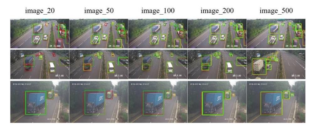
Figure 6 Visual comparison for object detection. Red: Ground truth, green: SSD, yellow: YOLO.
The saLFIA tool could successfully generate specified annotation files in YOLO or Pascal VOC format. Manual corrections can be performed using LabelImg, a manual annotation tool, to improve the generated annotation files. We could assess the impact of the number of initial images on detection accuracy based on the measurement results. SSD proved to be a better model than YOLO when fewer images were available. However, YOLO achieved maximum accuracy with a larger number of initial images. Consequently, the effort required for manual annotation can be gradually reduced by leveraging automatic detection from previously trained initial models.
4 Conclusions
The saLFIA pipeline operates through a command-line interface and consists of three main functions: image crawling from live-feed data, object detection using two methods, and automatic generation of annotation files. The user can specify the number of images, the storage location, and the source image URL via input parameters. The pipeline incorporates YOLOv3 and SSD as object detection algorithms, generating annotation files in either YOLO or Pascal VOC format following object detection.
Evaluation results indicate that YOLOv3 outperformed SSD when using a larger number of initial images, with only 8 misdetections. Conversely, SSD
demonstrated superior accuracy with fewer initial images, specifically with only 20 images. YOLOv3, however, achieved higher accuracy with a data set of 500 initial images. Increasing the total number of initial images reduced the need for corrective actions on the annotation files. Future studies will focus on improving both YOLOv3 and SSD detection algorithms to enhance the effectiveness of saLFIA in generating accurate annotations.