
1 Introduction
Antennas with a broad bandwidth, compact profile, and ease of mass production offer solutions for several developments in wireless communications devices and their conformance testing. Telecommunication technology that is currently actively operating on a broader frequency range, even up to the millimeter-wave (mmWave) spectrum, requires antennas that are capable of supporting it [1][2]. Simultaneously, the growing sophistication of telecommunications technology also brings the need for antennas that can function as sensors for testing the radiation characteristics of devices or electromagnetic compatibility (EMC). One of the requirements that must be met by an antenna that functions as a sensor in this test is a sufficiently wide bandwidth; the wider the bandwidth, the more straightforward the testing process that needs to be gone through [3]. As an added value, a compact form offers ease in carrying out the intended measurements or tests, in particular when it is conducted on a mobile device or a portable measuring device [4][5].
Optimization techniques are often required in the planning or design of a sensor. Popular optimization techniques, using different algorithm approaches, include genetic algorithm (GA), particle swarm optimization (PSO), and covariance matrix adaptation–evolution strategy (CMA-ES) [6]. In [7], GA was utilized to synthesize a microstrip antenna capable of quadband operation for mmWave applications with an observation range from 25 GHz to 65 GHz. The configuration reported in the study yielded four working bands, namely 27.9 GHz to 28.8 GHz, 37.1 GHz to 39.4 GHz, 45.9 GHz to 47.5 GHz, and 57.8 GHz to 64.5 GHz. Similarly, GA has also been applied to design a MIMO antenna desired to be able to operate from 3.1 GHz to 10.6 GHz [8].
Furthermore, the performance of GA and PSO in designing electromagnetic devices has been discussed in [9][10]. In line with these discussions, the performance of GA and PSO to improve the bandwidth of an E-shaped sensor for hyperthermia applications is presented in [11] and to improve the radiation pattern of conformal antenna arrays for mmWave and terahertz (THz) communications in [12]. The involvement of PSO in developing a desirable multi-band characteristic sensor has been implemented on a circular ring-shaped antenna with a fractal configuration in [13]. This technique was used to configure a planar monopole antenna to produce ultra-wideband (UWB) performance for short-range communications in [14]. A study comparing PSO with CMA-ES used in the design of electromagnetic sensors to obtain the desired multi-band response is reported in [15]. Moreover, in [16], CMA-ES was involved in designing UWB characteristic sensors that focus on improving the axial ratio of antenna array arranged aperiodically while maintaining an impedance bandwidth greater than 2:1.
Sensors with a spline-based configuration have been developed primarily to obtain wideband responses. By utilizing optimization techniques such as GA, PSO, and CMA-ES to determine the curvature control point on the spline can provide bandwidth responses or other desired radiation characteristics with a simpler process. For example, [17] presents a UWB antenna design that works in a frequency range from 3.1 GHz to 12 GHz and was oriented towards miniaturization of its physical size. The arrangement of a spline geometry involving GA is discussed in [18], where the designed antenna successfully
provided good bandwidth performance in a frequency range from 2.92 GHz to 14.9 GHz. Moreover, PSO was involved in configuring the spline curve, producing an antenna operating in a frequency range from 2.33 GHz to 20 GHz and from 3.7 GHz to 9.2 GHz at a reflection coefficient (S11) limit of less than –10 dB [19][20]. In addition, the reliability of CMA-ES in assisting a splinebased antenna configuration has also been reported [21]. This technique successfully improves bandwidth performance, resulting in a working range of 2.9 GHz to 20 GHz.
While optimization-based approaches have been widely applied in spline-based antenna design, most prior works examined GA, PSO, or CMA-ES individually, or compared only two techniques under different sensor structures. As a result, no systematic comparison has been done of GA, PSO, and CMA-ES within a single design framework for the same spline-based planar sensor configuration. This paper addresses that gap by directly comparing the three optimization techniques under identical design conditions to evaluate both bandwidth performance and optimization efficiency. At the end of discussion, the best configuration of optimization results is evaluated for realization. A bandwidth measurement of the realized planar sensor was performed to validate the simulation results, which are accompanied by several results of its radiation patterns and gains.
2 Planar Sensor Configuration
The spline curve is formed between two knot points, which are called the starting knot, located at the local coordinate center point, and the ending knot, located at the endpoint or tip of the patch, as shown in Figure 1(a). The patch of the proposed planar sensor is formed by utilizing a quadratic Bezier spline based on Eq. (1).
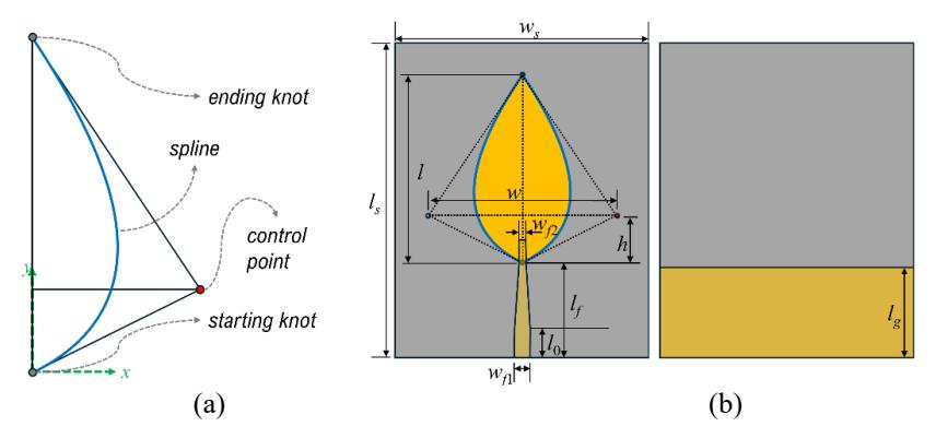
Figure 1 (a) Spline geometry involved in the planar sensor configuration and (b) physical parameters of the planar sensor.
\[B(t) = (1-t)^{2} P_{0} + 2t(1-t)P_{1} + t^{2}P_{2}\] (1)
It can be explained from Eq. (1) that B(t) is the point on the curve at parameter t, where t is a parameter that varies from 0 to 1. While \(P_0\) is the starting knot, \(P_1\) is the control point, and \(P_2\) is the ending knot.
The initial planar sensor configuration was built on Rogers RT/Duroid 5880 material with dimensions of 50 mm × 40 mm and a thickness of 1.57 mm. This material has a dielectric constant of 2.2 and a dissipation factor of 0.0009. The planar sensor had two copper laminated parts on the front side, namely the patch and the feedline; on the back side, there was a partial ground plane behind the feedline, as shown in Figure 1(b). The local coordinate center of the spline-based patch configuration was at the end of feedline, that is, 15 mm (\(l_f\)) from the base. The position of the control point in the patch configuration is represented by h and h0. By utilizing a symmetrical patch plane, the position of the control point will be at (h0/2,h1). The length between the starting and ending knots is represented by h1. The microstrip feedline has a tapered configuration, with the width at the base of h1 and the width at the end of h2. On the back side of the planar sensor, there is a partial ground plane with length h3 from the base.
To obtain the placement of the dynamic control point in the patch configuration, two variables in the design were used in associating parameters w and h as a function of l, namely \(r_1\) and \(r_2\), respectively, as expressed in Eq. (2):
\[w = \frac{l}{r_1}, \quad h = \frac{l}{r_2}. \tag{2}\]
Furthermore, Table 1 presents the dimensions of the parameters used in the initial configuration. Some of these parameters were later optimized to obtain the configuration that provides the widest bandwidth. Some parameters used in the optimization process were l, the control point position represented by \(r_1\) and \(r_2\), and the widths of the tapered feedline \(w_{l1}\) and \(w_{l2}\).
Table 1 Summary of the physical parameters in the initial configuration.
| Parameter | Length or Unit | Parameter | Length or Unit |
|---|---|---|---|
| \(l_s\) | 50 mm | \(l_f\) | 15 mm |
| \(w_s\) | 40 mm | \(l_0\) | 4.52 mm |
| l | 30 mm | \(l_g\) | 14.3 mm |
| \(w_{f1}\) | 2.4 mm | \(r_1\) | 1 |
| Wf2 | 1.0 mm | \(r_2\) | 4 |
3 Optimization Scenarios
Three types of optimization techniques were used to find the configuration of the planar sensor that produces the widest bandwidth, namely genetic algorithm (GA), particle swarm optimization (PSO), and covariance matrix adaptation—evolution strategy (CMA-ES). All three techniques were used in determining the values of the following physical parameters: l, \(r_1\), \(r_2\), \(w_{f1}\), and \(w_{f2}\). A general flowchart of the optimization scenarios using GA, PSO, or CMA-ES is shown in Figure 2.
The general optimization scenario includes the limit of increasing or decreasing the value of parameters l, \(r_1\), \(r_2\), \(w_{f1}\), and \(w_{f2}\) by 50% from the initial value so that the resulting patch and feedline configuration will not exceed the fixed-sized dielectric substrate area. Optimization using GA, PSO, and CMA-ES uses the cost function shown in Eq. (3).
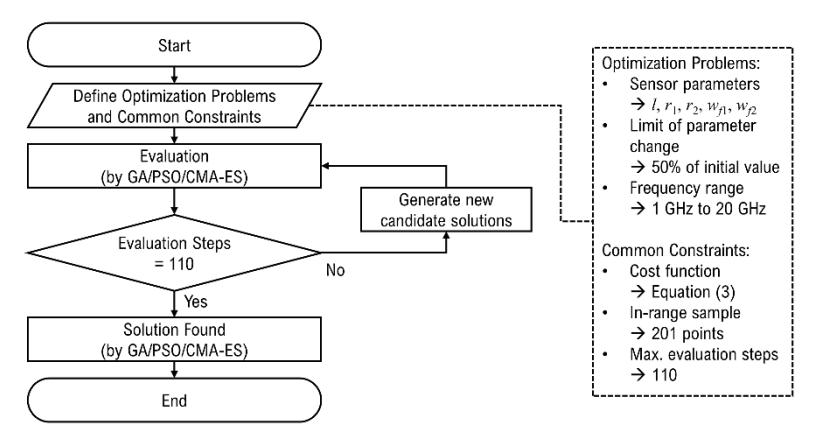
Figure 2 General flowchart of optimization scenario.
Cost = \[\sum_{f=1 \text{ GHz}}^{f=20 \text{ GHz}} C_f \cdot |S_{11}(f) + 13 \text{ dB}|\] (3)
The cost function is evaluated from 1 GHz to 20 GHz, which is linearly sampled at 201 points within the frequency range. Then, criterion \(C_f\) is equal to 1 if the \(S_{11}(f)\) value is higher than or equal to -13 dB and 0 if the \(S_{11}(f)\) value is smaller than -13 dB at each evaluated sampling frequency. The value of \(|S_{11}(f)| + 13\) dB| is the absolute value of the difference between the \(S_{11}\) at frequency f and -13 dB. The \(S_{11}\) value of -13 dB was used as the threshold in planning through simulation to provide the margin for realization of the planar sensor. As for the results of determining the bandwidth value at the end of simulation, the \(S_{11}\) threshold of -10 dB was still used.
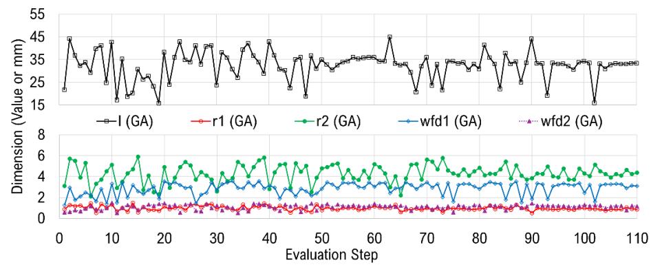
Figure 3 Changes in the values of the optimized parameters in the GA optimization evaluation steps.
Table 2 Comparison of the physical parameter values of the initial configuration and the optimization results using GA.
| Parameter | Initial Length or Unit | GA-optimized Length or Unit |
|---|---|---|
| l | 30 mm | 33.26 mm |
| r1 | 1 | 0.94 |
| r2 | 4 | 4.11 |
| wf1 | 2.4 mm | 3.20 mm |
| wf2 | 1.0 mm | 1.25 mm |
3.1 Genetic Algorithm
In this planar sensor optimization, GA was set using a population size of 4 × 5 and a maximum number of iterations of 10. The number of solver evaluations was 110, with a mutation rate of 60%. The GA optimization was completed in 10 hours, 14 minutes, and 17 seconds. Figure 3 shows the changes in the values of the optimized parameters in 110 evaluation steps. The parameter values resulting from the optimization process compared to the values in the initial configuration can be seen in Table 2. In sequence, the values of parameters l, r1, r2, wf1, and wf2 produced were 33.26 mm, 0.94, 4.11, 3.20 mm, and 1.25 mm.
3.2 Particle Swarm Optimization
In this optimization, PSO was set using a swarm size of 11 and a maximum number of iterations of 10, so the number of solver evaluations was 110 with a random seed of 1. Optimization using PSO took 10 hours, 3 minutes, and 57 seconds. Figure 4 shows the changes in the values of the optimized parameters in the 110 evaluation steps. The parameter values resulting from the optimization process using PSO compared to the values in the initial configuration can be seen in Table 3. As the solution, the values of parameters l, r1, r2, wf1, and wf2 produced were 33.99 mm, 1.03, 3.89, 3.24 mm, and 1.05 mm, respectively.
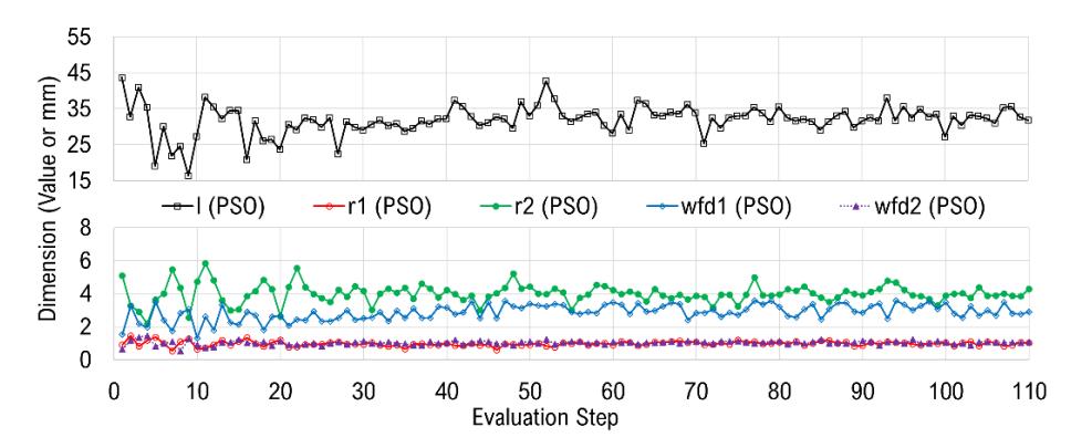
Figure 4 Changes in the values of the optimized parameters in the PSO optimization evaluation steps.
Table 3 Comparison of the physical parameter values of the initial configuration and the optimization results using PSO.
| Parameter | Initial Length or Unit | PSO-optimized Length or Unit |
|---|---|---|
| l | 30 mm | 33.99 mm |
| r1 | 1 | 1.03 |
| r2 | 4 | 3.89 |
| wf1 | 2.4 mm | 3.24 mm |
| wf2 | 1.0 mm | 1.05 mm |
3.3 Covariance Matrix Adaptation–Evolution Strategy
The planar sensor optimization using CMA-ES was done through 110 evaluations, a random seed of 1, and a sigma value 0.5. Optimization using CMA-ES took 10 hours, 58 minutes 53 seconds. Figure 5 shows the changes in the values of the optimized parameters in the 110 evaluation steps. The parameter values resulting from the optimization process using CMA-ES compared to the values in the initial configuration can be seen in Table 4. The resulting parameter values of l, r1, r2, wf1, and wf2 were 32.97 mm, 0.84, 5.32, 3.34 mm, and 1.50 mm, respectively.
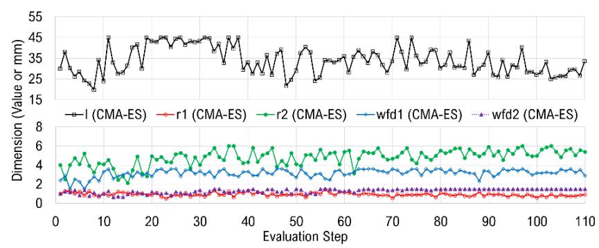
Figure 5 Changes in the values of the optimized parameters in the CMA-ES optimization evaluation steps.
Table 4 Comparison of the physical parameter values of the initial configuration and the optimization results using CMA-ES.
| Parameter | Initial Length or Unit | CMA-ES-optimized Length or Unit |
|---|---|---|
| l | 30 mm | 32.97 mm |
| \(r_1\) | 1 | 0.84 |
| \(r_2\) | 4 | 5.32 |
| \(w_{f1}\) | 2.4 mm | 3.34 mm |
| \(W_{f2}\) | 1.0 mm | 1.50 mm |
4 Comparison of Optimization Results
All optimization techniques used had 110 evaluations. Figure 6 shows the changes in the values of each parameter l, \(r_1\), \(r_2\), \(w_{f1}\), and \(w_{f2}\) that occurred during the evaluation steps carried out through optimization using GA, PSO, and CMA-ES. Moreover, Figure 7 presents a visualization of the configuration changes in the half-plane of the planar sensor surface at the initial condition against the optimization results using GA, PSO, and CMA-ES.
The normalized cost was used to compare the performances of the three optimization techniques. The normalized cost value was obtained from Eq. (4):
\[Cost_{norm} = \frac{Cost - Cost_{min}}{Cost_{max} - Cost_{min}}.\] (4)
In each optimization technique, the normalized cost value, Cost<sub>norm</sub>, is the normalization of the actual cost value obtained from Eq. (3) against the minimum cost, Cost<sub>min</sub>, and the maximum cost, Cost<sub>max</sub>, which are the lowest and highest cost values of all the evaluation steps performed. The lowest normalized cost with a value of 0 throughout the optimization performed in 110 steps indicates the step position that produces the configuration with the widest bandwidth.
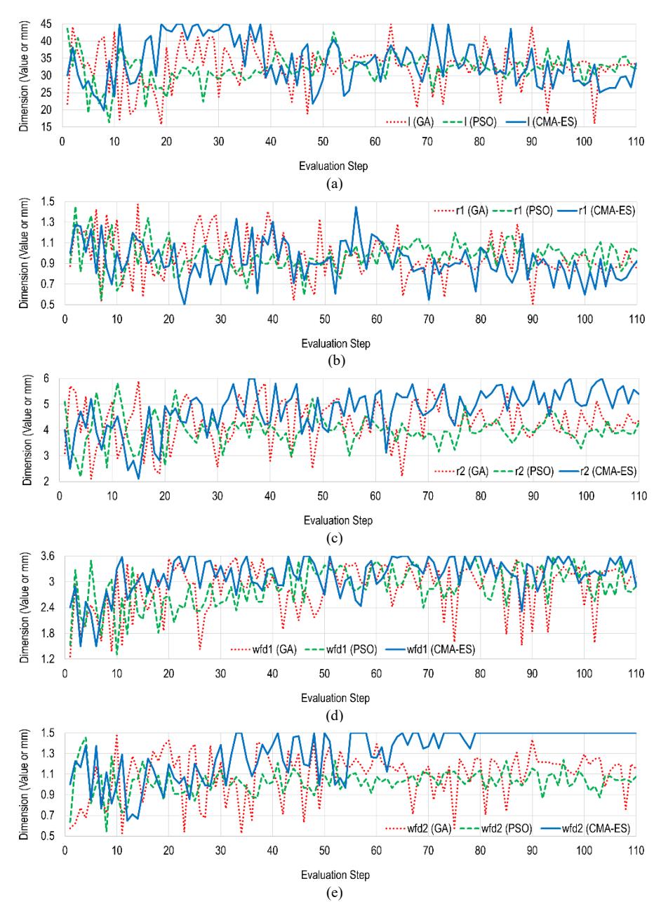
Figure 6 Comparison of the changes in values of (a) l, (b) r1, (c) r2, (d) wf1, and (e) wf2 in the GA, PSO, and CMA-ES optimization evaluation steps.
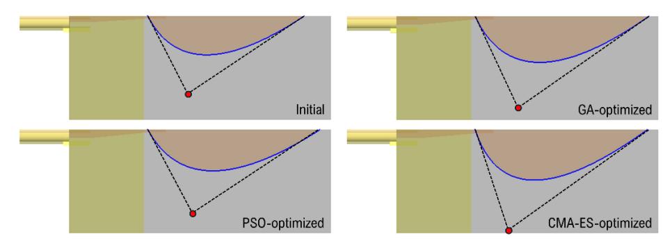
Figure 7 Visualization of the configuration changes in the half-plane of the planar sensor surface at the initial condition against the optimization results using GA, PSO, and CMA-ES.
Figures 8, 9, and 10 each present the normalized cost achieved throughout the evaluation steps using GA, PSO, and CMA-ES, respectively. From the three normalized cost graphs, GA obtained the optimal value at the 76th step, PSO at the 66th step, and CMA-ES at the 58th step of the 110 steps performed. In general, it can be observed that the convergence of the normalized cost with a value approaching zero was more dominant in the optimization performed using PSO. This is supported by the average normalized cost value, which occurred at a value of 0.114 when compared to GA and CMA-ES, which each had values of 0.174 and 0.201.
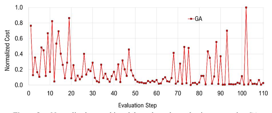
Figure 8 Normalized cost achieved throughout the evaluation steps using GA.
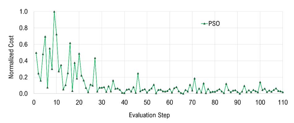
Figure 9 Normalized cost achieved throughout the evaluation steps using PSO.
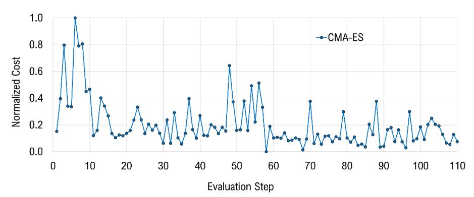
Figure 10 Normalized cost achieved throughout the evaluation steps using CMA-ES.
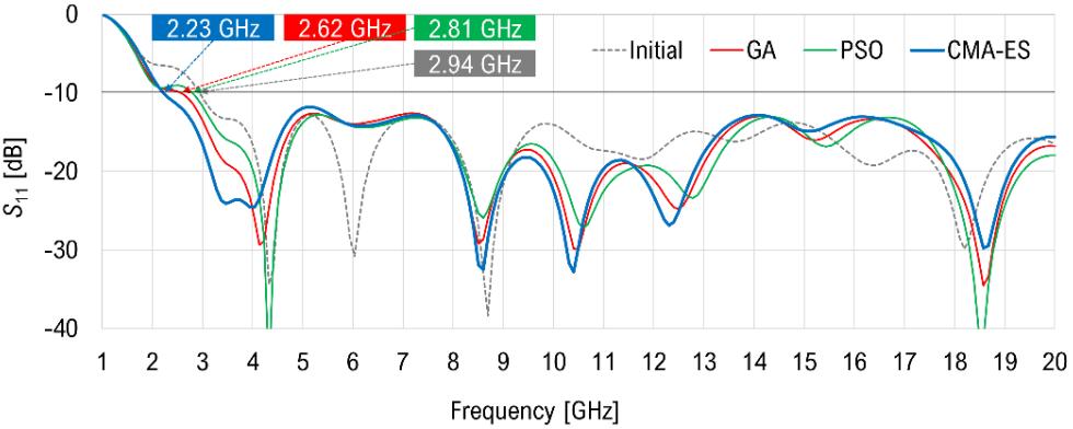
Figure 11 Comparison of the S11 response of the initial configuration and the optimal configurations produced by GA, PSO, and CMA-ES.
| Performance | GA | PSO | CMA-ES |
|---|---|---|---|
| Mean of Costnorm | 0.174 | 0.114 | 0.201 |
| Time (hours:minutes:seconds) | 10:14:17 | 10:03:57 | 10:58:53 |
| Frequency range (GHz) | 2.62-20 | 2.81-20 | 2.23-20 |
| Bandwidth (GHz) | 17.38 | 17.19 | 17.77 |
| Geometric bandwidth | 240.1% | 229.3% | 266.1% |
Table 5 Performance comparison of GA, PSO, and CMA-ES in optimizing the planar sensor configuration.
Figure 11 compares the \(S_{11}\) response of initial configuration with the optimal configurations resulting from optimization using GA, PSO, and CMA-ES. Using the \(S_{11}\) threshold reference of -10 dB, the initial planar sensor configuration had a working range from 2.94 GHz to 20 GHz. Comparing the working range, the configurations resulting from optimization using GA, PSO, and CMA-ES, respectively, had a working range from 2.62 GHz to 20 GHz, 2.81 GHz to 20 GHz, and 2.23 GHz to 20 GHz. It was seen that optimization using CMA-ES produced the planar sensor with the widest bandwidth. By using Equation (5), the geometric bandwidth obtained from the configurations resulting from optimization using GA, PSO, and CMA-ES was determined:
\[BW_{geom} = \frac{f_h - f_l}{\sqrt{f_h \times f_l}} \times 100\%.\] (5)
The geometric bandwidth, \(BW_{geom}\), is a percentage of the difference between the higher frequency, \(f_h\), and the lower frequency, \(f_l\), to the geometric mean of its bandwidth. The geometric bandwidth obtained from the configurations of each optimization result with GA, PSO, and CMA-ES was 240.1%, 229.3%, and 266.1%, respectively.
Table 5 compares the optimization performance using GA, PSO, and CMA-ES to finalize the configuration. Based on the mean of the normalized cost, as discussed in the previous section, supported by the graphs presented in Figure 8 to Figure 10, PSO provided a better value. However, this also shows that the deviation of changes in the optimized parameter values was not as wide as for GA or CMA-ES, which can also be seen in Figure 6. Moreover, considering the time consumed to complete all steps in the optimization process, PSO took less time compared to GA or CMA-ES. On the other hand, although slower by 54 minutes 56 seconds than PSO and 44 minutes 36 seconds than GA, optimization using CMA-ES provided the planar sensor configuration with the broadest bandwidth among the three, that is, 17.7 GHz from the frequency range of 2.23 GHz to 20 GHz, or a geometric bandwidth of 266.1%.
From the comparison results shown in Table 5, the advantages and disadvantages of each optimization technique can be studied. PSO provides time efficiency, and CMA-ES produces better final results, in this case providing the most expansive bandwidth, which is the priority. Between the two, GA provides the position between PSO and CMA-ES that balances time efficiency and bandwidth results. Based on the comparison between optimization through GA, PSO, and CMA-ES, the configuration that was realized in this study was the one produced by CMA-ES.
5 Planar Sensor Performance and Analysis
The configuration obtained from CMA-ES optimization was realized using the Rogers RT/Duroid 5880 substrate. Previously, to ensure that dimensional shifts due to uncertainties in the etching process would not cause significant differences in the S11 response, fabrication feasibility was carried out through simulations by enlarging or reducing the dimensions of the copper laminate on the dielectric substrate to ±1% of the actual size. The results of the dimensional shift test can be seen in Figure 12, which shows that the decrease or increase in the lower frequency was relatively minimal and did not produce an upper frequency limit until the end of observation window, at 20 GHz. Furthermore, Figure 13 presents the planar sensor that was realized, accompanied by the measuring instruments and anechoic chamber facilities that were used to verify the results of the simulations that were carried out and to find out information on the radiation pattern and gain produced by the planar sensor.
Furthermore, the results of this measurement were then compared with the simulation results that had been carried out. The results of the measured S11 response of the spline-based planar sensor can be seen in Figure 14. The measurement results show that the configured planar sensor had a slightly wider bandwidth. When compared with the simulation results, the planar sensor had a working range from a frequency of 2.23 GHz to 20 GHz, while the realized planar sensor had a working range from a frequency of 2.14 GHz to 20 GHz, or a geometric bandwidth of 273%.
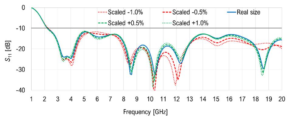
Figure 12 Fabrication feasibility testing through simulation to determine the effect of copper area scaling on the planar sensor.
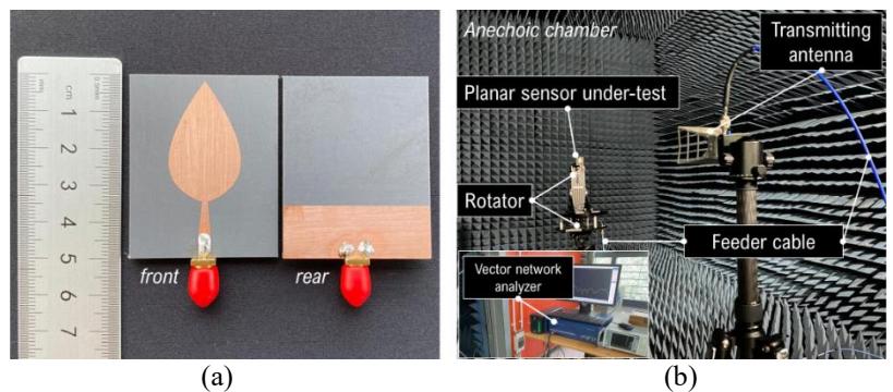
Figure 13 Photographs of (a) the realized planar sensor configuration and (b) its measurement setup.
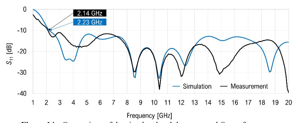
Figure 14 Comparison of the simulated and the measured S11 performances.
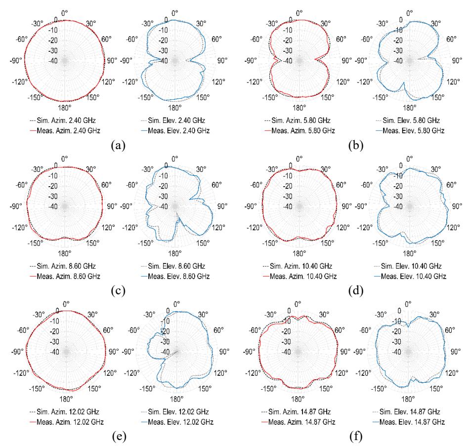
Figure 15 Comparison of the simulated and the measured radiation patterns at (a) 2.40 GHz, (b) 5.80 GHz, (c) 8.60 GHz, (d) 10.40 GHz, (e) 12.02 GHz, and (f) 14.87 GHz in the azimuth and elevation planes.
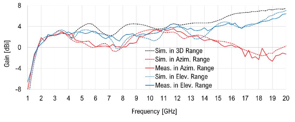
Figure 16 Comparison of the simulated and measured gain.
Figure 15 compares the radiation pattern of the simulation and the measurement results at commonly used applicative frequencies and the frequencies where the S11 minima response occurred. The frequencies displayed in the radiation pattern measurement are 2.40 GHz, 5.80 GHz, 8.60 GHz, 10.40 GHz, 12.02 GHz, and 14.87 GHz. In relation to Figure 15, the radiation patterns at these frequencies are also compared in the azimuth and elevation planes. Generally, the radiation pattern at lower frequencies tends to approach omnidirectional and then gradually becomes more directive at higher frequencies. In addition, it can also be concluded that good agreement between the simulation and the measurement results was achieved. Moreover, to obtain additional information on the radiation characteristics of the planar sensor, gain measurements in the azimuth and elevation planes were carried out. As shown in Figure 16, the gain generated from the antenna varied throughout the observed frequency range, with the maximum gain occurring in the elevation plane at a frequency of 20 GHz, that is, 7.05 dBi based on the simulation results and 6.43 dBi based on the measurement results. In the higher frequency region, it can be observed that the gain generated by the planar sensor was more dominant in the elevation plane. This result indicates that the directivity of the radiation pattern at high frequencies occurs on the axis in the feedline direction on the planar sensor.
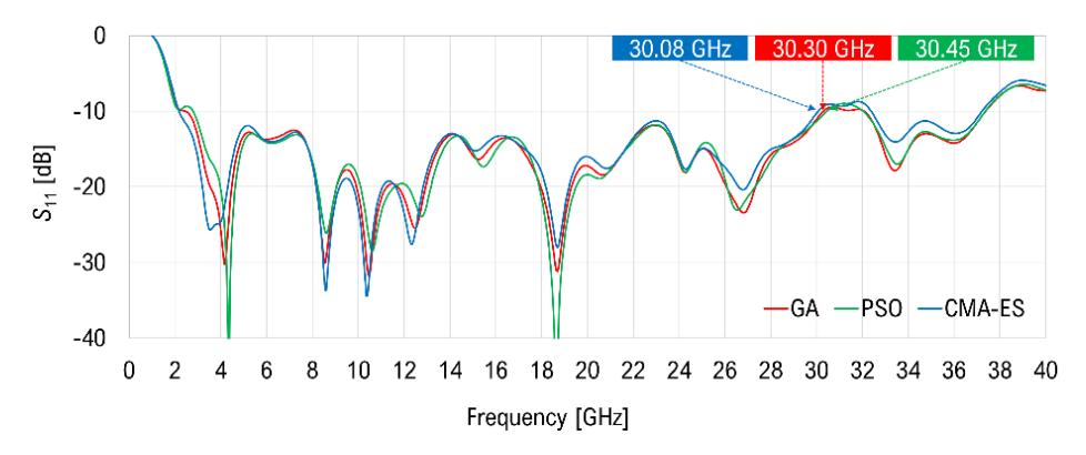
Figure 17 Extended comparison of bandwidth performance.
Due to the limit of the measurement equipment, the characterization was restricted to 20 GHz. To provide further insight, we extended the analysis up to 40 GHz by simulation for the GA-, PSO-, and CMA–ES optimized designs. Within the optimization range of 1 GHz to 20 GHz, the respective operating ranges were 2.62 GHz to 20 GHz (GA), 2.81 GHz to 20 GHz (PSO), and 2.23 GHz to 20 GHz (CMA-ES). Up to the observation frequency limit adjusted to the measurement instrument's capabilities, 20 GHz, all configurations still maintained their S11 response below –10 dB. Therefore, to determine the upper frequency limit of each planar sensor configuration, the simulation was extended from 1 GHz to 40 GHz, encompassing the L, S, C, X, Ku, K, and Ka bands. Figure 17 presents the S11 responses of each configuration resulting from optimization within this extended bandwidth observation. When extended to 40 GHz, the working ranges became 2.62 GHz to 30.30 GHz (27.68 GHz bandwidth, GA), 2.81 GHz to 30.45 GHz (27.64 GHz bandwidth, PSO), and 2.23 GHz to 30.08 GHz (27.85 GHz bandwidth, CMA-ES). Although CMA-ES produced a slightly lower upper frequency compared to GA and PSO, it still achieved the broadest overall operating bandwidth. Using the geometric bandwidth, the highest to lowest gains were 340%, 310.7%, and 298.8% for the configurations using CMA-ES, GA, and PSO, respectively. These gains are for additional information only, considering that the optimization process was conducted with evaluations ranging from 1 GHz to 20 GHz only.
6 Conclusion
A performance comparison of optimization techniques using GA, PSO, and CMA-ES in configuring a spline-based planar sensor to enhance its bandwidth was presented in this paper. PSO generally provides an optimization completion speed advantage, while CMA-ES offers better bandwidth results. GA positioning is in between both rein terms of process completion speed and bandwidth. The geometric bandwidths produced by GA, PSO, and CMA-ES were 240.1%, 229.3%, and 266.1%, respectively. Since the optimized configuration with the broadest bandwidth was achieved by CMA-ES, this model was realized for performance validation. In the simulated configuration of CMA-ES, the planar sensor working range was from a frequency of 2.23 GHz to 20 GHz, while the validation showed a working range from 2.14 GHz to 20 GHz, or a geometric bandwidth of 273%. With the wide bandwidth and good radiation characteristics achieved, the planar sensor presented is worthy of consideration because of its suitability to support testing of EMC and wireless communications. In addition, with the presentation of extended observations up to a frequency of 40 GHz, the bandwidth performance of the spline-based planar sensor discussed in this study may be continued in terms of configuration, measurement verification, and modification in the future.