
1 Introduction
Organizations or companies have assets that support their operations, such as tools and equipment. One of the critical issues in the modern era is fast or even real-time, asset detection, known as the Real Time Location System [1-5]. Hospitals represent highly dynamic environments where medical assets are frequently moved across departments, such as emergency units, intensive care units, and inpatient rooms under time-critical conditions. Items urgently needed by the organization should be located quickly. In a hospital setting, assets or equipment can be required with urgency daily [5]. Various technologies have been used for asset detection or tracking in the modern era. One of them is RFID technology. Studies on the use of RFID in hospitals and other healthcare contexts have been widely conducted [6, 7]. The healthcare industry widely adopts RFID because it enables automatic, non-line-of-sight identification, does not require manual scanning, and can operate reliably in indoor environments where continuous asset availability is critical. Moreover, RFID systems allow scalable deployment with relatively low cost and minimal operational disruption, making them suitable for large and complex hospital environments. By considering technological, organizational, and environmental factors, hospitals can utilize RFID to improve efficiency, service quality, and operational management [6].
Alternative technologies such as Global Positioning System (GPS), Bluetooth Low Energy (BLE), Ultra-Wideband (UWB), and Wi-Fi-based positioning have also been explored for real-time location systems. However, GPS is not suitable for indoor environments due to signal attenuation, while BLE and Wi-Fi typically require higher infrastructure density and calibration to achieve acceptable accuracy. UWB provides high positioning accuracy but involves higher deployment and maintenance costs, making it less practical for large-scale hospital asset tracking. Therefore, this study focuses on RFID-based asset monitoring, which offers a balanced trade-off between cost, maturity, indoor feasibility, and deployment complexity.
In the healthcare industry, several problems include a lack of tracking and tracing capabilities, inefficient data capture, human error in business processes, and nonintegrated data management systems [8]. These problems lead to medical mistakes, increasing costs, theft, loss, and inefficient workflow [8]. The US Food and Drug Administration (FDA) estimates that medical errors occur in 40% of manual or paper-based environments [9]. In addition, it is estimated that 10% of medicines in a typical hospital are lost each year due to theft [1].
A concrete example of this problem can be observed in hospital equipment relocation scenarios. Critical medical devices such as ventilators, infusion pumps, or defibrillators are frequently moved between patient rooms, emergency units, intensive care units, and storage areas based on immediate clinical needs. In emergency situations, medical staff often require these assets within minutes. However, due to manual recording, delayed system updates, or inaccurate asset tracking, equipment may be reported to incorrect locations, leading to longer search times and delayed patient care. In some cases, staff members manually relocate equipment without updating the inventory system, further increasing the risk of false location information. This scenario highlights the necessity of an automated, real-time, and reliable asset tracking system in healthcare environments.
From a technological point of view, the architecture of an RFID for healthcare asset monitoring can consist of tags, readers, and gateways, as shown in Figure 1 [2].
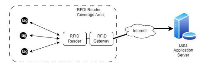
Figure 1 Overview of RFID architecture for asset tracking [11].
The results of RFID tag readings are sent to the data application server [11, 12]. Tags are placed on each asset to facilitate reading. There are various forms and configurations of RFID usage on assets. This research proposes using a fixed reader and a dynamic passive tag. Dynamic means that certain assets can be moved under certain conditions. For example, a ventilator can be moved from one room to another in a hospital. In this scenario, the reader is placed permanently in one room, while the tag is attached to an asset that can be moved at any time. In an actual deployment, asset location data is obtained from passive RFID tags attached to each asset and transmitted to the server via fixed readers. In this study, a simulation-based approach is used; therefore, RFID readings and asset movements are generated using probabilistic and stochastic models whose statistical characteristics emulate realistic hospital asset movement patterns.
With this architecture, assets can be monitored in real time. RFID reading operates in polling mode initiated by the reader. Then, the RFID reading is sent to the server [13]. If polling is done frequently, sending server data causes other problems, such as delays or traffic collisions. In a traffic collision, the average response time increases due to the large amount of data sent concurrently to the server [14, 15]. Too frequent polling is also considered harmful, because it increases battery consumption, especially for battery-powered RFID readers. On the other hand, if polling is too rare, the system's ability to detect becomes less accurate. Assets that have moved but have not been updated again are in the wrong room. In this study, this condition is referred to as false identification. Therefore, it is necessary to determine the right time to poll so that the goal is still achieved.
Based on the above considerations, the core problem addressed in this study is to determine the optimal RFID polling interval, which balances conflicting system objectives. Excessively frequent polling increases the network load, communication delays, and reader energy consumption, while infrequent polling
leads to outdated asset location information and longer false-identification times. In healthcare environments where asset availability is time-critical, an inappropriate polling strategy can negatively impact both system performance and operational effectiveness.
This study proposes an optimization method to determine the most suitable period in polling data. Some aspects considered include minimizing delay or network load, maximizing reader energy efficiency, and minimizing the average time of false identification. This approach can be categorized as a Multi-Objective Problem (MOP) problem. The weighted-sum method, combined with Monte Carlo simulation, can find the optimal value. A Monte Carlo simulation assesses the uncertainty in asset movements and how the proposed model responds to these dynamics. This uncertainty can later be modeled as a probability distribution with a given average and variance of asset movement.
This paper contributes to the existing literature by formulating the RFID polling interval selection problem in hospital asset tracking as a multi-objective optimization problem that explicitly considers conflicting system objectives. Unlike prior studies that typically adopt fixed or heuristic polling configurations, this study introduces a quantitative definition of false identification duration to capture the impact of delayed asset location updates caused by infrequent polling. Furthermore, a simulation-based evaluation framework using Monte Carlo methods is developed to model stochastic asset movements and assess system performance under different polling strategies. By integrating information accuracy, reader energy consumption, and network response time into a unified weighted-sum optimization model, this study provides a systematic and reproducible approach for determining an optimal polling interval in RFID-based healthcare asset monitoring systems.
2 Related Work
2.1 Asset Identification & Tracking
Asset identification and tracking are essential processes in an organization's asset management, especially for organizations with many productive, distributed assets [16, 17]. Some organizations are facing trust issues with the asset registers they maintain, with inaccuracy rates reaching 5% [18]. One of the core problems in asset identification is the inability to maintain up-to-date and accurate asset location information, particularly when assets are frequently moved without timely system updates. Asset identification is not just about gathering basic asset information; it also requires identifying the asset's history and locating or positioning it. Therefore, it allows the organization to track and manage its assets efficiently. Finding assets in buildings, such as equipment and components, becomes more challenging as buildings are larger and more complex [19]. This challenge is further amplified in hospital environments, where assets are highly mobile and urgently required within short time windows. Various techniques have been developed to support this process, from conventional methods to modern technologies such as RFID (Radio Frequency Identification) [20]. Likewise, the use of RFID in hospitals has also begun to develop [9]. This technology can be combined with the Internet of Things to send data to the server [21].
Technologies such as barcodes and RFID have been leveraged to provide information regarding asset location, status, condition, and maintenance history, resulting in a 30.8% increase in asset utilization [12]. Although this technology remains expensive, several factors can accelerate the adoption of RFID in hospitals [6, 7]. Several surveys have stated that automatic monitoring mechanisms are widely approved [22]. Various items can be tracked using RFID, including patients, assets, drug containers, and medical supplies [8]. The use of real-time tracking can help reduce search time [23].
2.2 Energy Efficient Issue in RFID
Energy efficiency is indeed one of the issues to consider in the use of RFID [13, 24]. A key problem arises from the polling-based operation of RFID readers, where frequent scanning is often used to improve asset visibility but leads to excessive energy consumption and increased communication overhead. While several strategies have been proposed to reduce energy usage, including optimizing communication protocols between tags and readers and implementing more energy-efficient hardware designs [24], there still remains a fundamental trade-off between energy efficiency and system performance. However, despite advances, challenges remain in balancing energy efficiency with operational range or system accuracy [25]. This trade-off is especially critical in healthcare environments, where RFID readers are expected to operate continuously and reliably, making energy-efficient polling strategies essential for sustainable and scalable deployment [26].
2.3 RFID Architecture Deployment
The use of RFID for asset tracking or indoor location has led to various system architectures. Supporting the needs of many identified assets can be done using a multiple-tag approach [21]. Such architectures also often use passive RFID (passive tags) to be placed or attached to the assets. In addition, an antenna or RIFD scanner can detect whether an asset is in the room. The general architecture is shown in Figure 1 by Adame et al. [11]. The results of the RFID reading are sent to the server [11, 12].
Scanning over longer distances can use UHF RFID [9, 20, 27]. Polycarpou et al. used UFH RFID tags and UHF RFID scanners placed in specific places [9, 20]. Further development can be done by combining RFID with BIM to help improve the indoor location accuracy of assets [27]. One architectural approach is to place an RFID reader near the entrance door to detect asset movement as they enter or leave the room [28].
Another approach using passive tags can be combined with reference tags. These reference tags are used to locate other tags, thereby reducing the burden on the Real Time Location Service (RTLS) [29].
2.4 Multi-objective Optimization
Real-world problems, such as those in hospitals, can be included in the Multi-Objective Problem (MOP) category [1]. Multi-objective optimization can solve MOP problems involving multiple objective functions [30]. In the context of RFID and RTLS applications, this multi-objective optimization can be applied to balance energy-efficiency requirements and tracking accuracy, thereby mitigating false identification and network load. This approach enables problemsolving by considering multiple conflicting factors to produce a more holistic, appropriate solution for complex operational conditions, such as in hospital environments.
Several research examples have developed MOP optimization. One of these is to increase productivity and reduce costs and energy consumption in autonomous industrial processes by minimizing robot arm working time, travel time, and energy use while maximizing global business profits [31]. In the context of the building industry and energy-efficient renovation efforts, the MOP approach has been developed to minimize retrofit costs, energy consumption, and emissions while maximizing thermal comfort [32]. Another case study used a multiobjective approach to optimize COVID-19 patient admissions in hospitals, considering admission time and readiness, and used the Pareto Optimization algorithm to select the most appropriate hospital, thereby increasing efficiency and saving patient lives [30].
3 Method
In this section, the model developed in this study is discussed. The first part explains the proposed system architecture. Next, several relevant terms in this model are introduced. The optimization model aims to obtain the optimal scanning period in the next part.
3.1 Conceptual Model & System Architecture
The model developed in this study prioritizes a fixed reader position in a particular room. In this study, an RFID system wasimplemented that used passive UHF RFID tags compliant with the EPC Gen2 (ISO 18000-6C) standard, operating in the 860-960 MHz frequency band. Fixed UHF RFID readers equipped with directional antennas are assumed to be deployed at predefined locations within hospital zones, specifically near room entrances, to ensure reliable detection of asset movement between rooms. Considering typical indoor hospital environments, the effective reading range of each reader was conservatively assumed to be approximately 5 meters.
RFID tags are attached to each movable asset, such as medical equipment that is frequently relocated during daily hospital operations, including ventilators and heart monitors. These assets may move from one room to another depending on clinical needs. To illustrate this operational scenario, Figure 2 conceptually represents the relationship among fixed readers, moving tags, and room-level asset identification.
Figure 2 depicts a simplified hospital layout consisting of multiple rooms, each equipped with a fixed RFID reader. The black circles represent RFID tags attached to assets, while the square icons indicate fixed readers assigned to specific rooms. The dashed arrows represent asset movement across rooms over time. This illustration is not intended to represent a specific hospital floor plan, but rather to visually explain the fundamental detection mechanism assumed in the proposed model.
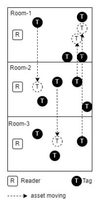
Figure 2 Illustration of fixed RFID readers and moving tags.
Therefore, at a given time, , tag is detected by reader . Since reader is fixed and uniquely associated with a specific room, the detection event directly
implies that the asset is located within the room at that time. By continuously monitoring tag–reader associations, the system can infer asset transitions between rooms as discrete movement events.
This room-based detection mechanism enables the development of a location identification system without requiring precise coordinate-level localization. Such an approach is particularly suitable for hospital environments with multiple rooms and floors, where room-level accuracy is often sufficient for operational decision-making. Knowing the exact room location of an asset can reduce search time, improve asset utilization, and enable more efficient transfers according to clinical demands.
3.2 How It Works
In this paper, it is proposed that one reader be assigned to a specific room. In the room, some assets have been equipped with passive tags. The reader actively requests tags according to the EPC Gen2 or ISO 18000-6C protocol [3]. The tag responds to the reader with an EPC or ID. Figure 3(a) illustrates the logical architecture of this process, in which the reader collects identification data from multiple passive tags within its coverage area and forwards it to the server to update asset location information. The server acts as a centralized component that maintains the latest known position of each asset based on the reader's fixed location, which corresponds to a specific room. Figure 3(b) further explains how reader–tag interaction occurs over time by illustrating the basic communication protocol and the temporal structure of the scanning process.
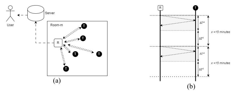
Figure 3 Protocol communication between an RFID reader and passive tags, (a) architecture, (b) basic protocol communication.
The communication protocol generally starts with the reader querying the tag, which then responds with a specific ID. This process can be done in batches for multiple tags: the reader queries them simultaneously and the tags respond simultaneously. With this concept, the system can have scanning and idle periods (neither active nor scanning). In Figure 3, a grey block depicts the active period, and the active scanning time is denoted by ∆ . After that, the reader enters an idle period until the next active period. This idle period is the idle duration, or with the notation ∆ . The total scanning duration is denoted by x. The illustration in Figure 3 uses a scanning duration of 15 minutes and serves only as a visualization example.
To provide a simpler picture, from a time-series perspective, the communication protocol can be represented as shown in Figure 4. In each scanning duration (x), there are two periods: the period for active scanning (∆ ) and the period for idle (∆ ) in Eq. (1).
\[x = \Delta T = \Delta T^A + \Delta T^I \tag{1}\]
One cycle of the scanning period is denoted by p, which spans periods 2 and 3 through P. To carry out observations for 150 minutes with a scanning duration of, for example, 15 minutes, the number of cycles is 150/15 = 10.
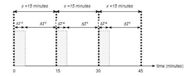
Figure 4 How protocol communication works in a time series.
3.3 Simulation Setup and Evaluation Procedure
This study adopted a simulation-based evaluation approach to analyze the performance of the proposed RFID asset tracking model and its associated optimization framework. The simulation represents a hospital indoor environment in which multiple assets equipped with passive RFID tags move between rooms monitored by fixed RFID readers.
The simulation environment consisted of a set of rooms, each equipped with a UHF RFID reader installed near the room entrance. Assets carry passive UHF RFID tags and may enter or leave rooms over time. RFID readers periodically initiate scanning processes according to a scanning duration , following the EPC Gen2 (ISO 18000-6C) communication protocol described in Section 3.2. All identification results are transmitted to a centralized server that updates the asset location information.
The system configuration included a fixed number of tagged assets, fixedposition RFID readers, and a backend server. The scanning duration was treated as the decision variable and was varied within a predefined range, while other parameters were held constant in each simulation scenario.
The evaluation procedure was conducted using a Monte Carlo simulation to capture the stochastic nature of asset movements and identification events. Asset movement behavior was modeled as a stochastic process, in which movement events for each asset were generated using random variables with predefined means and variances. The mean represents the average asset movement frequency, while the variance captures heterogeneity in asset mobility across different asset types. These statistical parameters were intended to emulate realistic hospital asset movement characteristics rather than represent a deterministic physical process.
For each candidate scanning duration, multiple simulation runs were performed over a fixed observation horizon. During each run, three performance metrics were recorded: mean false identification time, RFID reader energy consumption, and network response time. The metric values were averaged across the simulation runs and used as inputs to the multi-objective optimization model.
3.4 False Identification
The identification process from the reader to the tag is certainly not carried out every second with certain considerations, as explained in the previous section. The identification process can be carried out every 15, 30, or 60 minutes, depending on needs. However, overly long identification can lead to false identification. An example of this is in Figure 5. For example, identification was carried out every 15 minutes. At 15.15, asset A was identified in room number 2. However, during the idle duration at 15.20, asset A was moved to room number 10. Users who checked the system at 15.25 saw that asset A was still in room 2, even though it had been moved, resulting in a false identification. The new information was corrected when it was updated at 15.30. This condition is called false identification. The duration from the occurrence of false identification to the next scanning period is called the duration of false identification (∆ ).
In the previous example, the scanning time used was 15 minutes. In practice, the scanning is set to occur every 15, 30, or 60 minutes based on the needs. Scanning periods that are too fast are considered less effective because they involve several considerations, such as excessive battery usage and too frequent data traffic (leading to overruns when updating asset position information). If it is too long, it will lead to incorrect information about the current asset position.
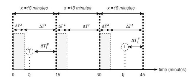
Figure 5 False identification.
3.5 Tag Moving Rate
In real-world environments, such as hospitals, asset movement does not occur as frequently as in manufacturing. However, some assets move more frequently than others. Assets used frequently, such as IV poles and thermometers, are moved more often than assets such as beds. Likewise, beds are moved more frequently than assets such as cabinets. Using historical data, the average time to move assets can be determined using RFID tags. This parameter is referred to as the Tag Moving Rate, denoted by ∆().
Monte Carlo simulation was used in the research to describe the movement of assets (tags). For example, there are three assets with asset movement data as follows:
- 1. Asset A: 2 times a week
- 2. Asset B: 1 time a week
- 3. Asset C: 3 times a week
An example of the movement and transfer of assets with Monte Carlo simulation is shown in Figure 6. In this example, two results were generated from a distribution by generating random times of asset movement.
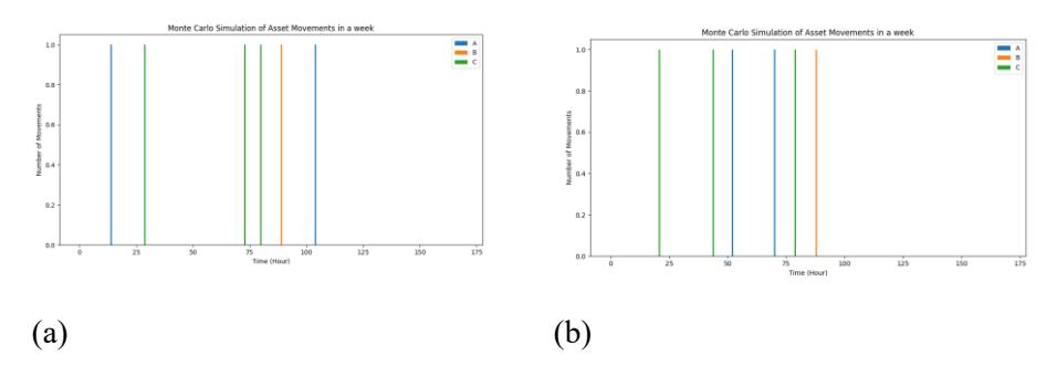
Figure 6 Illustration of asset transfer with Monte Carlo simulation: (a) example for 1st generation of random data, (b) example for 2 nd generation of random data.
The architecture of the proposed system is that the reader, after gaining information, sends data to the data center. Data delivery is performed sequentially after the asset is successfully scanned. To reduce the risk of false identification, delivery to the server can be done as often as possible. However, this can also have other impacts. Network performance decreases and server performance load increases. In previous studies, the more concurrent users there are on the server, the more the system performance decreases. For example, the response time is longer. To solve this problem, the effect of the number of concurrent users on performance is modeled as follows:
\[R(u) = \frac{M}{1 + e^{-k(u - u_0)}} \tag{2}\]
The function ()represents the response time as a function of the number of concurrent users , where denotes the maximum response time, determines the steepness of the curve, and 0is the number of concurrent users at which the response time reaches half of the maximum value .
Eq. (2) defines the response time function, (), using a logistic growth model (or sigmoid function) that characterizes the non-linear relationship between system performance and user load. In this context, the system's latency is modeled as a function of the number of concurrent users, , where represents the upper asymptote or the theoretical maximum response time the system reaches under saturation. The parameter determines the logistic growth rate, signifying how abruptly the response time degrades as the load increases, while 0 identifies the inflection point of the curve—the specific user threshold where the response time reaches exactly half of its maximum value (/2). This model is particularly robust for performance engineering, as it captures the transition from stable operations to a saturated state, providing a predictable framework for scalability analysis and network capacity planning.
An example visualization of this modeling, using the response-time parameters summarized in Table 1, is shown in Figure 7.
Table 1 Parameters of the Response-Time Model.
| Parameter | Symbol | Value |
|---|---|---|
| Maximum response time | (M) | 30 s |
| Steepness factor | (k) | 0.004 |
| Inflection point | (𝑢0) | 1000 users |
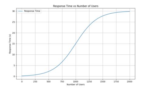
Figure 7 Visualization of modeling the influence of the number of concurrent users on the average response time.
3.6 Energy Consumption Measurement Model
Energy consumption in this study was estimated based on the operational states of the RFID reader, namely the active scanning and idle periods. Since passive UHF RFID tags do not contain an internal power source, the energy consumption considered in this model solely refers to the RFID reader.
During the active period (∆ ) the reader continuously transmits interrogation signals and receives tag responses according to the EPC Gen2 protocol. The reader is assumed to consume a constant active power (in watts). Conversely, during the idle period (∆ ), the reader remains powered on but does not actively interrogate tags, resulting in a lower idle power consumption (in watts).
The energy consumption per scanning cycle is calculated using the following formulation:
\[C(x) = P_A \cdot \Delta T^A + P_i \cdot \Delta T^I \tag{3}\]
The function ()represents the energy consumption per cycle expressed in joules (J), where denotes the active power, represents the idle power, Δ is the duration of the active period, and Δ is the duration of the idle period.
Eq. (3) illustrates the cumulative energy consumption per scanning cycle, C(x), formulated as the sum of the energy dissipated during two distinct operational states: the active and idle phases. The model employs a power-time product approach, where . ∆ represents the energy consumed while the system is actively processing or scanning, and . ∆ accounts for the energy overhead during the inactive or standby interval. By integrating these discrete power levels over their respective durations, the equation provides a precise quantification of the resource utilization in joules (J). This modeling approach is fundamental for assessing the energy efficiency of scanning cycles, as it allows researchers to identify which operational state contributes most significantly to the total power
budget, thereby facilitating optimization for low-power or battery-constrained environments. C(x) is the energy consumption per cycle expressed in joules (J). For reporting convenience, energy consumption over the observation period is accumulated across all cycles and converted to watt-hours (Wh).
In the simulation, \(P_A\) and \(P_i\) were treated as fixed parameters derived from typical commercial UHF RFID reader specifications, while the scanning duration x directly determined the proportion between \(\Delta T_A\) and \(\Delta T_i\). This approach allows the impact of scanning frequency on reader energy consumption to be systematically evaluated.
3.7 Optimization Objective Function
This study proposes the development of an optimization model with certain objective goals. This study uses a multi-objective function with the following objective functions:
- 1. Minimize the average duration of false identification
- 2. Minimize the total power consumption of the reader
- 3. Minimize the response time for data sent from the reader to the cloud server. The decision variable is related to the reader scanning period (x). Therefore, the function of each objective function on each asset (asset m) can be explained as follows:
The first objective function (f1) is as follows:
\[f_1^m(x) = \mathcal{C}(x) \tag{4}\]
\[f_1^m(x) = \frac{\sum_{i=1}^{P} \Delta T_i^F(x)}{P}\] (5)
The function \(f_1^m(x)\) represents the first objective function, which measures the average false identification time for asset m, where \(\Delta T_i^F(x)\) denotes the duration of false identification time in cycle i, and P is the total number of cycles during the observation period.
The first objective function, denoted as \(f_1^m(x)\) in Equations (4) and (5), quantifies the average false identification time for a specific asset $m$ throughout the observation period. As formulated in Equation (5), the function is calculated by taking the summation of the false identification durations, \(\Delta T_i^F(x)\), and dividing it by the total number of cycles, P. This mathematical approach provides a normalized metric for system inaccuracy, in which the numerator aggregates the temporal errors across all i cycles. Furthermore, the values for these durations are generated using a Monte Carlo simulation to account for the stochastic nature of degradation. By optimizing the results of Equation (5), the model effectively minimizes the time the system spends in an erroneous state, thereby enhancing the overall diagnostic reliability of the asset monitoring framework. Random degeneration was simulated using a Monte Carlo simulation to generate values.
The second objective function (f2) is as follows:
\[f_2^m(x) = \sum_{i=1}^{p} C(x)\] (6)
\[C(x) = \begin{cases} C_a. a & if & active period \\ C_i. (x - a) & if & idle period \end{cases}\] (7)
The function \(f_2^m(x)\) represents the second objective function, which measures the total energy consumption during the observation period normalized by \(a \times P\) for the m-th asset, where C(x) denotes the energy consumption in each cycle, composed of \(C_a\) as the energy consumed during the active period \((\Delta T^A)\) and \(C_i\) as the energy consumed during the idle period \((\Delta T^I)\), and are presents the duration of the active period in minutes.
The second objective function, represented as \(f_2^m(x)\) in Equation (6), calculates the total energy consumption for the m-th asset by aggregating the individual energy costs of each cycle, C(x), over the entire observation period P. The specific energy consumption for each cycle is further defined in Equation (7) through a piecewise formulation that distinguishes between active and idle states. In this context, \(C_a\) represents the energy consumed during the active period, where a denotes the active duration in minutes, while \(C_i\) accounts for the energy dissipated during the remaining idle interval. By summing these components as shown in Equation (6), the model provides a comprehensive metric for the system's power demand, enabling optimization of operational parameters to balance performance and energy efficiency.
The third objective function (f3) is as follows:
\[f_3^m(x) = \frac{M}{1 + e^{-k(u - u_0)}} \tag{8}\]
\[u = P \tag{9}\]
The function \(f_3^m(x)\) represents the third objective function, which measures the response time for asset m, where M denotes the maximum response time (a constant), k represents the steepness of the curve (a constant), u is the number of concurrent users or connections during the period, and \(u_0\) is the number of concurrent users at which the response time reaches half of the maximum value M.
The third objective function, defined as \(f_3^m(x)\) in Equation (8), characterizes the system response time for asset m using a logistic growth framework. In this formulation, the parameter M represents the maximum constant response time under saturation, while k signifies the steepness constant of the response curve. The variable u, which denotes the number of concurrent users or connections within a given period, is set equal to the total number of cycles P as specified in Eq. (9). Furthermore, \(u_0\) is the critical threshold at which the response time reaches exactly half of its asymptotic maximum value. By integrating these parameters into Eq. (8), the model effectively maps the non-linear degradation of system performance as the user load increases, providing a quantitative basis for maintaining service-level objectives within the monitoring framework. The number of concurrent users or connections can be approached by the number of cycle periods. In each cycle period, there is a connection to the data delivery to the server.
The function applies to each asset. When added up, it gives the sum of all assets. The equation for each objective function is as follows:
\[f_1(x) = \sum_{i}^{M} f_1^{m}(x) \tag{10}\]
\[f_2(x) = \sum_{i}^{M} f_2^{m}(x) \tag{11}\]
\[f_3(x) = \sum_{i}^{M} f_3^m(x) \tag{12}\]
To produce equivalent values, the three values of the function are normalized. The function for the combination of the three functions becomes as follows:
\[F(x) = minimize \left[ w_1. f_1(x) + w_2. f_2(x) + w_3. f_3(x) \right]\] (13)
The parameters \(w_1\), \(w_2\), and \(w_3\) represent the weights assigned to the first, second, and third objective functions \((f_1, f_2, \text{ and } f_3)\), respectively, indicating their relative importance in the overall evaluation.
The system-wide performance is evaluated by aggregating the results of each objective function across all M assets, as defined in Eqs. (10), (11), and (12). These values are then integrated into a single objective function F(x) = in Eq. (13) using a weighted-sum approach, which is to be minimized. In this formulation, \(w_1\), \(w_2\), and \(w_3\) represent the specific weights assigned to the first objective function \((f_1)\), the second objective function \((f_2)\), and the third objective function \((f_3)\), respectively. These weights are crucial for determining the relative importance of each metric, allowing the model to balance trade-offs between false identification time, energy consumption, and response time based on operational priorities.
To determine the optimal polling time, the decision variable is evaluated over a predefined discrete range reflecting practical operational settings in hospital environments. For each candidate polling time, Monte Carlo simulations are conducted to capture stochastic asset movements and identification events over a fixed observation period. The three objective functions—average false identification duration, total reader energy consumption, and system response time—are calculated and averaged across simulation runs. Due to the conflicting nature of these objectives, all objective values are normalized and aggregated using a weighted-sum approach as defined in Eq. (12). The optimal polling time is defined as the polling interval that minimizes the combined objective function (), representing the best trade-off among information accuracy, energy efficiency, and system responsiveness under the given assumptions.
4 Result & Discussion
This section explains the results of running these functions. The simulation was run using a Monte Carlo method to find the optimal periodic scanning time (x). The search window started from x = 0 to x = 10,080 minutes, or approximately one week. The best periodic scanning time was selected based on the optimum value of the three functions, as explained in the previous section. The parameter values used to obtain the results in this section are summarized in Table 2.
| Parameter | Symbol | Value |
|---|---|---|
| Number of assets | M | 100 (varied) |
| Scanning period range | x | 10,080 minutes |
| Mean moving rate | μ | 2.48 |
| Variance | σ² | 0.7896 |
| Max response time | M | 30 s |
| Steepness | k | 0.004 |
| Inflection point | u₀ | 1000 users |
| Active power | Pₐ | 20 W |
| Idle power | Pᵢ | 5 W |
Table 2 Parameter Settings for the Monte Carlo Simulation.
4.1 Results
The trend of each objective function can be seen in the movement of one of them. For this test, an example is provided with 100 assets, an average moving rate parameter of 2.48, and a variance of 0.7896. For f1, the trend movement is depicted in Figure 8. The f1 function shows the change in the average duration of false identification over the scanning period, as shown in Figure 8. The higher the scanning period (variable x), the higher the average false identification, and this relationship is linear. This is aligned with the observation that the longer the scanning period, the higher the false duration. This result indicates that increasing the polling interval directly lengthens the time lag between actual asset movement and system awareness, leading to prolonged periods during which assets are reported at incorrect locations. Therefore, Figure 8 provides quantitative evidence that infrequent scanning significantly degrades the accuracy of location information, highlighting false identification duration as a critical objective to minimize in the proposed multi-objective optimization framework.
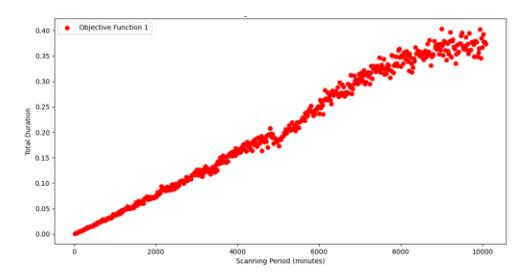
Figure 8 Relationship between scanning period time and average false identification duration.
The f2 function shows the average change in total energy consumption over the scanning period, as shown in Figure 9. The higher the scanning period (variable x), the lower the average total energy consumption, following a negative logarithmic trend. This is aligned, since the longer the scanning period, the longer the idle time, which lowers energy usage.
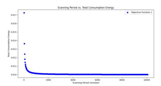
Figure 9 Relationship between scanning period time and total energy consumption on the reader.
The f3 function shows the change in the average response time for data delivery over the scanning period, as shown in Figure 10. The higher the scanning period (variable x), the lower the average total response time, with an S-shaped curve. This aligns with the idea that the shorter the scanning period, the more requests and responses are needed to send data to the cloud, increasing the average response time. When the scanning period is longer, the number of data delivery requests is lower, so the average total response time is shorter. Therefore, given the three objective functions, the optimal value lies in the middle. The optimum value is the lowest (minimization) combination of the three values. The figure shows the changes in the three functions with the same weighting. Each weight was 0.33. The result is given in Figure 11.
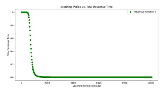
Figure 10 Relationship between scanning period time and average response time.
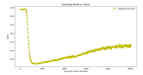
Figure 11 Results of period scanning of the combination of the three functions with the same weight (0.33).
In the function, there are global maxima and minima. Since the global minimum is used, it is taken at the point where the figure starts to decline. The rebound point, when it reverses to the top, is the global minimum; in the simulation, it was reached at x (scanning period) = 1460 minutes, or approximately 24.3 hours. In this case, the best scanning period, according to calculations for 100 assets with an average of 2.48, is approximately 24.3 hours or one day. Thus, the system can use periodic scanning to send data every 24.3 hours to achieve the optimal value.
4.2 Discussion
This section explains aspects of the model's sensitivity to parameter changes. Some parameters were kept constant, while others were changed. The test results show the changes in the decision variable (x).
4.2.1 Effect of the Number of Assets on the Decision Variable
This chart shows the effect of changes in the number of assets on the decision variable (x), or on the scanning period variable. Some other parameters were kept constant, such as the average moving rate of 2.5 and the variance of 1. The result of this test is given in Figure 12.
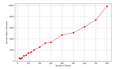
Figure 12 Effect of the number of assets on the decision variable.
Figure 12 shows that increasing the number of assets also increases the decision value (scanning period). The difference between the minimum and maximum values is 9340 minutes, or about 155 hours. From this difference in value, the number of assets significantly affects the variable x.
4.2.2 Effect of Average Moving Rate on the Decision Variable
This scenario was conducted by testing several values of the average moving rate while keeping the number of assets and the variance of the moving rate constant. Thus, the effect of the average moving rate on the decision variable (x) or on the scanning-period variable is evident. Some other parameters were kept constant, such as the average number of assets (100) and the moving rate variance (1). The test results for various average moving rates are shown in Figure 13.
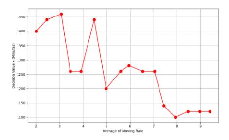
Figure 13 Effect of the average moving rate on the decision variable.
In Figure 13, as the average moving rate increases, the decision value (scanning period) decreases, though not significantly. The decision to take the value of variable x is not very significant. The difference between the lowest and highest values is only 360 minutes or about 6 hours.
4.2.3 Effect of Moving Rate Variance on the Decision Variable
This scenario was conducted by testing several values of the moving-rate variance while keeping the number of assets and the average moving rate constant. Thus, the effect of the moving-rate variance on the decision variable, or scanning-period variable (X), could be observed. Low variance indicates that the moving rate is close to its average, while high variance indicates that the moving rate is increasingly variable. For the test sample, the other parameters were kept constant: the average number of assets was 150, and the moving rate was 5. The test results for various moving rate variances are shown in Figure 14.
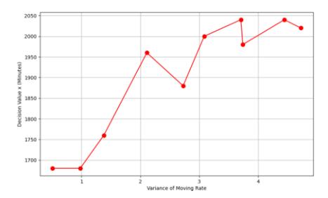
Figure 14 Effect of moving rate variance on the decision variable.
Figure 14 shows that, with higher variance, the decision value (scanning period) is higher, though not significantly so. This relates to organizations with very diverse or highly variable asset transfers. The decision to take the value of the variable x is not very significant. The difference between the lowest and highest values is only 350 minutes or about 5.8 hours.
4.2.4 Effect of Weighting One of the Objective Functions on the Decision Variable
This scenario was carried out by trying several weight values against the second function. The values of the number of assets, average moving rate, and variance moving rate were the same. Thus, the effect of the weight value on the decision variable (x) or the scanning period variable is evident. The first step is the effect of the f1 weight.
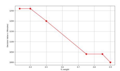
Figure 15 Effect of the weight of f1 on the decision variable.
In Figure 15, a higher f1 weight corresponds to a lower decision value (scanning period), though not significantly. If the focus shifts to the duration of false identification, the scanning period can be reduced.
In the next step, the values that was changed was the weight of f2. The result is given in Figure 16.
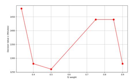
Figure 16 Effect of the weight on f2 on the decision variable.
In Figure 16, the higher the weight of f2, the less impactful the decision value (scanning period). This means that focusing more on energy consumption does not significantly affect decision-making. In the next step, the changed value was the weight of f3; the result is shown in Figure 17.
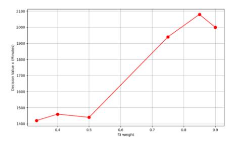
Figure 17 Effect of weight on objective f3 on the decision variable.
In Figure 17, a higher f3 weight corresponds to a higher decision value (scanning period), though not significantly. This means that if we focus more on network performance, we can extend the scanning time.
4.2.5 Using Two Objective Functions on the Decision Variable
This section discusses what happens when the model only uses two functions. The first simulation only used f1 and f2, so the weight for f3 was set to 0. Similar to the previous one, this step also examined the effect of weighting: if one weight is in one function, the other is lowered. The result is shown in Figure 18.
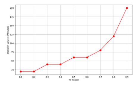
Figure 18 Effect of the weight of f2 on the decision variable.
In Figure 18, a higher f2 weight corresponds to a higher decision value (scanning period). This aligns, since the duration period (x) must be longer to focus on energy consumption. Without considering f3, the x variable falls within a narrow range of 25 to 200 minutes.
In the second part, only f1 and f3 are used, with f2 weighted by 0. The result is given in Figure 19.
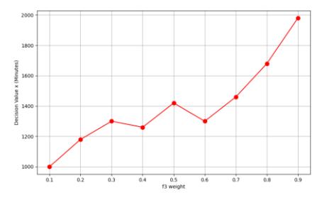
Figure 19 Effect of the weight of f3 on the decision variable.
In Figure 19, the higher the value of the weight of f3, the higher the decision value (scanning period). This means that by focusing on network performance, the duration (x) must be longer.
The experimental results show that several factors, including the number of assets, the average moving rate, and the moving-rate variance, influence the selection of the scanning period in an RFID system. The simulation results indicate that the optimal scanning period for 100 assets, with an average moving rate of 2.48, is approximately 24.3 hours. This time is obtained by analyzing three objective functions, each contributing differently to the decision-making. Considering all functions, the global minimum value is achieved, indicating that combining these three variables is vital in determining the optimal scanning time.
The sensitivity analysis results for variations in the number of assets show that the increase is directly proportional to the required scanning time. This indicates that organizations with more assets should be prepared to extend the scanning time to optimize monitoring. In contrast, the effect of the average moving rate on scanning time is insignificant, although a downward trend is observed. This means this factor should be optimized but not be the focus of decision-making.
Moving rate variance also contributes to scanning time, with the trend that higher variance requires longer scanning time. This underscores the importance of considering the stability of asset movement when designing an efficient system. In addition, the weighting of the objective function also affects the results. Placing greater weight on the false identification duration function reduces scan time, whereas focusing on network performance increases it.
Finally, this study confirms that to achieve optimal performance, system developers need to consider all these factors. Given the varied dynamics of asset usage, the right decision on scanning time will ensure operational efficiency and reduce energy costs in RFID systems. System developers need to consider multiple interrelated factors when designing RFID-based asset tracking systems in healthcare environments, including polling interval selection, reader energy consumption, network communication load, and the accuracy of asset location information. These factors are tightly coupled with real-world operational conditions, as asset movements are driven by dynamic clinical workflows and urgent medical demands rather than deterministic system behavior. Consequently, the impact of system configuration choices extends beyond technical performance and directly affects hospital operations. Therefore, the responsibility is not limited to system developers alone but also involves other stakeholders such as hospital management, IT operators, and medical staff, whose usage behavior, workflow patterns, and operational constraints influence asset mobility and system effectiveness. This interaction between technical parameters and human-driven processes explains why inappropriate polling strategies can lead to longer false-identification durations, higher energy consumption, or delayed asset availability, highlighting the need for a holistic, stakeholder-aware optimization approach.
5 Conclusion
This paper identified challenges in asset detection within the healthcare industry, particularly delays and inaccuracies arising from suboptimal RFID polling methods. This study proposes an optimization method to determine the optimal polling period that balances network delay, reader energy efficiency, and the average false identification time. The conclusions of this study were derived from a multi-objective optimization analysis and simulation-based evaluation under stochastic asset movement conditions, which allowed a systematic assessment of the trade-offs inherent in polling-based RFID systems. The results of one experiment showed that for 100 assets with an average moving rate of 2.48, the optimal scanning period was achieved at 1460 minutes. Experiments with variations were conducted to examine how the model responds to different variables spanning the scanning period. Sensitivity analysis revealed that increasing the number of assets is directly proportional to the scanning time, while the average moving rate has an insignificant effect. The variance of the moving rate also contributes; the higher the variance, the longer the required scanning time. The objective function weights indicate that focusing on the duration of false identification reduces scanning time, whereas focusing on network performance increases it. While this study focused on polling-related performance metrics to maintain model clarity and tractability, other factors, such as system scalability, deployment cost, reader placement density, and other considerations, may also influence real-world implementations and are identified as directions for future research. This study developed a holistic model to determine the optimal scanning time for achieving operational efficiency and reducing energy costs in RFID systems.
Acknowledgements
The authors would like to express their gratitude to Telkom University and the University of Western Australia for their financial support and collaborative facilities provided for this research. This work was conducted under a joint research framework funded by these institutions, which enabled the development and optimization of the mathematical models presented in this study. The authors also appreciate the technical assistance and academic environment that contributed to the completion of this research.