

1. INTRODUCTION.
We use variable diaphragms, in measuring magnitudes of stars on photographic plates by use of Eichner-photometers. We shall get erroneous results if the emulsion density of the background of the standard sequence and that of the stars of unknown magnitudes differ. Several authors (Argue 1960, Kwee 1962) have in the past tried to overcome this difficulty. A method however, which results in better approximations to the non-erroneous magnitudes, and which does not consume too much time, is badly needed. This paper presents a type of method which is applicable, regardless of the convenience of the relationships between photometer reading and some photometric quantities.
2. THEORETICAL BASIS.
The background effect in photographic photometry may be illustrated with Table 1, which lists magnitudes for the cluster NGC 6530 (Walker 1957), a nebulous cluster with pronounced background sky-fog. Magnitudes derived photoelectrically are compared with photographic determinations in which a sequence in the nearby cluster NGC 6531 (Hoag, et al., 1961) has been used. The latter cluster is not embedded in nebulosity, and can be photographed simultaneously with NGC 6530 in the plates used for the present study.
TABLE I. Correct versus Erroneous Magnitudes\nin NGC 6530.
| Walker's Star Number | \[\begin{array}{c} \text{Correct} \\ \text{m}_{\text{B}} \end{array}\] | Erroneous \(m_{\rm B}\) | ||
|---|---|---|---|---|
| 31 | 11.97 | 11.63 | ||
| 41 | 12.89 | 10.28 | ||
| 42 | 9.24 | 6.03 | ||
| 47 | 12.50 | 9.99 | ||
| 49 | 11.22 | 9.47 | ||
| 52 | 12.43 | 10.36 | ||
| 54 | 11.84 | 7.37 | ||
| 56 | 9.21 | 6.81 | ||
A brief description of the astrophotometer of the Warner and Swasey Observatory is given below before we consider the problem of background effect.
Two beams of light originating from the same source are compared in this photometer: one is transmitted through a variable iris-diaphragm which is varied by the measurer, then transmitted through the photographic plate on which the star image is measured. The other beam, called the comparison beam, goes through a diaphragm of constant diameter. The latter diaphragm may be changed, but for a given plate only one diaphragm is used. The relative intensity of the beams is measured by a photoelectric cell, and equality of intensity can be judged with the help of a cathode ray oscilloscope. The task of the measurer is to vary the iris diaphragm such that the flux of the variable beam equals the flux of the comparison beam, and this can be readily ascertained with the help of the oscilloscope. The star and iris images are projected on a viewer screen wherefrom the measurer is able to see whether the star image is well centered in the iris image.
The difficulty with an astrophotometer having a variable iris diaphragm is that we do not know the amount of flux which falls on the iris diaphragm before being transmitted through the plate. Numerical values of the astrophotometer reading as a function of the diameter of the iris diaphragm of the astrophotometer of the Warner and Swasey Observatory were found in unpublished data by Sanduleak. From graphical plots of his data the functional relationship of iris diaphragm diameter to photometer readings is
\[10^{R} = 1.49q + 0.88 \tag{1}\] where R= astrophotometer reading and q= diameter of iris diaphragm in inches. Thus it is possible to determine the relative flux crossing the iris at a given opening by making use of the astrophotometer readings, since by these readings we can derive the area of the iris diaphragm through which the flux is transmitted.
Let \(S_o\) be the area of the image of the iris diaphragm after a setting on an obscured region, let \(S_c\) be the area of the corresponding image of the iris diaphragm if the setting had been made on a part of the emulsion which is clear.
In similar fashion let \(S_{i,o}\) be the area of the star image measured in the obscured region, and \(S_{i,c}\) be the corresponding area for a measurement made in the clear emulsion. Then
\[(S_o - S_{i,o})F_{tr,o} = C_1\] (2)
\[(S_c - S_{i,c})F_{tr,c} = C_2 \tag{3}\] where \(F_{tr,o}\) and \(F_{tr,c}\) represent the transmitted flux through the obscured area and the clear area, respectively.
Divide the first equation by the second one, and assume that:
- (1) the scattering and absorption by the fictitious clear region is zero and thus \(F_{tr,c}\) equals the incident flux \(F_i\);
- \((2) \quad S_{i,o} = S_{i,c};\)
- (3) the intensity of the incident beam is equal throughout the beam cross-section;
- (4) the diaphragm is circular; and
- (5) \(C_1\) and \(C_2\) of Equations 2 and 3 are equal for varying \(S_0\), since these transmitted fluxes are made equal to that of the comparison beam which is presumably constant throughout the measurement.
The areas of the star images in the clear area, i.e. \(S_{i,e}\), do not differ much from the corresponding \(S_{i,o}\), although a slight difference exists. The effects of this difference will be eliminated by the trial and error procedure to be described.
\[\frac{(S_{o} - S_{i,o})}{(S_{c} - S_{i,c})} \cdot \frac{F_{tr,o}}{F_{i}} = 1\] (4)
By definition the second factor of the left-hand side is the transmission, T, of the obscured region. Since the density, D, of the emulsion can be expressed in terms of T by \(D = \log \frac{1}{T}\), equation 4 becomes.
\[S_{c} = 10^{-D}S_{o} + (1 - 10^{-D})S_{i,o}\] (5)
This is the formula which transforms the area of the projection on the plate of the iris diaphragm into the equivalent area if the region of the emulsion had been clear. Thus if we know \(S_{i,o}\), and D, the correction for the background effect is at hand. \(S_{i,o}\) is easily found by using a sequence of fly spanker images for which diameters have been measured. Scale readings can also be arranged on the screen on which the observer sees the images of the stars and the measuring diaphragm, so as to know directly the area of the star image.
3. APPLICATION.
For the present experiment, the diameters of the stars were measured with the astrometric machine, which is not the most convenient for the purpose. The diameters were then plotted against the known photoelectric magnitudes and a table of \(S_{i,o}\) as function of magnitude was then derived (see Fig. 1).
Next we consider the problem of determining the density. It is natural to look for an empirical relation, between astrophotometer readings and photographic densities. This has been done on the Warner and Swasey photometer by making use of a photographic wedge. The densities of an array of points on the wedge were measured by using a transmission densitometer. The same points were then measured in the astrophotometer. It turned out that a plot of astrophotometer readings versus density can be closely represented by a straight line. There is, however, a very slight deviation from the straight line plot at the smaller density end, if small comparison beam diaphragms are used. For larger ones no curving was observed. Since the correction will be mostly applied on dense nebulous regions, the straight line approximation is certainly sufficient. Before and after a measuring period with the astrophotometer, fixed points of known density on a wedge should be measured to establish the density photometer reading calibration and its constancy. Experience showed that one can
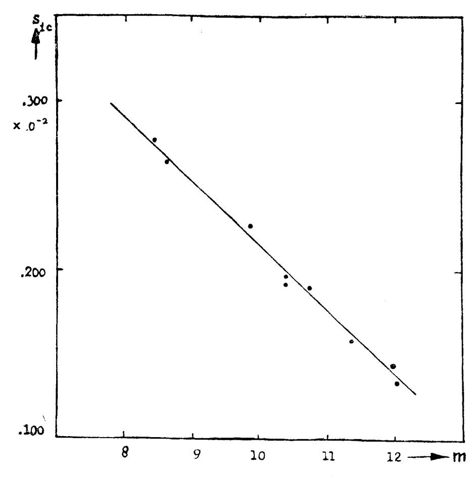
Fig. 1. Image Area and Magnitude.
easily forget and measure a point on the wedge twice if the screw to move the plate happens to be used up to its end. Therefore it is suggested that the measured points on the photographic wedge be marked with numbers, and that these numbers be observed during the readings. The plateholder of the astrophotometer may be so designed that the photographic plate and wedge can be measured interchangeably.
There is still the problem of determining the area \(S_o\) of the image of the iris diaphragm projected on the emulsion. It is convenient to derive \(S_o\) in terms of the astrophotometer readings R.
The principal difficulty is that we do not know the reduction of the iris diaphragm by the optical system which concentrates the measuring beam on the image of the star. This can be overcome empirically by trial and error.
To find the exact relationship between \(S_o\) and R we make use of Equation 5 and of a calibration curve (magnitudes versus R) for a sequence in a clear region. A trial and error procedure is then followed in which computed magnitudes are compared with observed photoelectric magnitudes until agreement is obtained.
In Equation 5, D and \(S_{i,o}\) are now known. To start with, an approximate \(S_o\) can be obtained by measuring the image of the iris diaphragm on the plate. This can be done, for example, on the projection screen if the star image diameter, already known is used as a unit. The actual area of the iris diaphragm, \(S_d\), can also be compared with the help of Equation 1, from the observed astrophotometer reading when \(S_o\) is measured. Hence the factor f, by which the optical system reduces the iris diaphragm diameter, can be obtained.
If we multiply \(S_d\) by \(f^2\), we obtain the area of the image of the iris diaphragm projected on the emulsion. Since for a given \(S_d\), R is known, we can now plot a curve which relates R with \(S_o\).
The factor f for the Warner and Swasey Observatory astrophotometer is 0.073. Thus \(f^2\) is 0.0053. A list of some of the values of \(S_d\) of this photometer is given below. \(S_d\) is in square inches.
TABLE 2. Reading versus Iris Area.
| R | \(S_d\) | |||
|---|---|---|---|---|
| .1500 | .08709 | |||
| .2000 | .16046 | |||
| .2500 | .27062 | |||
| .3000 | .42660 | |||
Multiplying \(S_d\) by. 0053 gives us values for reading versus iris image area (see Fig. 4, curve c).
As an illustration of the background correction we now give a stepby-step description of the method followed in the present study. In order to obtain the most accurate results, one should take measures to prevent temperature changes in the measuring room. For recording purposes, a minimum amount of room light should be allowed.
Do not use plates of uneven development, or plates requiring changes of focus of the astrophotometer during the measurements. Both NGC 6530 and NGC 6531 should be in the unvignetted area. It is advisable to use fine grain emulsions. Fogged plates should be discarded.
First Step. Measure with the astrophotometer the marked points of the photometric wedge and draw a plot of the already known densities of those points versus the readings, For the Warner and Swasey astrophotometer this plot is a straight line (Figure 2).
Second Step. Measure the star images of the clear cluster members, NGC 6531 in this case. (Fig. 3).
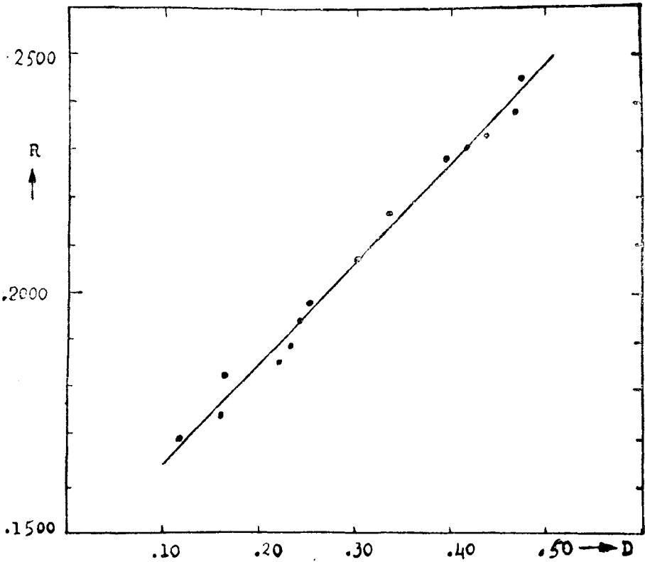
Fig. 2. Relationship between Astrophotometer Reading and Emulsion Density.
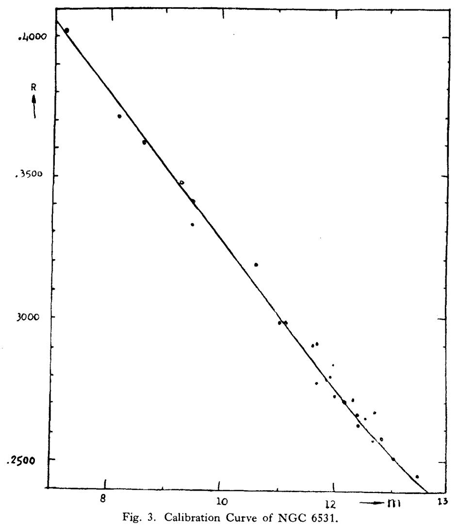
Third Step. Measure stars of known magnitudes in the nebulous cluster (NGC 6530). Besides measuring star images, measure the neighboring background at four or more points, by moving the image on the screen up and down or right and left. (The larger the background variations, the more points should be measured).
Fourth Step. Measure \(S_{i,c}\) for a set of stars of known magnitudes. The results for the present study have been presented already in Fig. 1. \(S_{i,c}\) and \(S_{i,c}\) are assumed to be equal for stars of given magnitude.
Fifth Step. First approximations for \(S_a\) are derived from Fig. 4, Curve C, and the readings obtained in Step 3.
Sixth Step. We now have values for D, \(S_{i,o}\) and a first approximation for \(S_o\). Substitute \(S_o\), D, and \(S_{i,o}\) into Equation 5 and obtain for each of the stars measured in NGC 6530, \(S_c\). This is approximately the iris image area that would result if the region were cleared of nebulosity. S. corresponds to a reading \(R_c\) which may be obtained with Fig. 2.
Seventh Step. From \(R_c\) derive magnitudes with the help of Fig. 3, which was obtained in Step 2. If the derived magnitudes do not equal the magnitudes of the stars, new approximations for \(S_c\) can be made, and the last two steps repeated until satisfactory agreement between computed and observed magnitudes is obtained.
After the first approximation the magnitudes resulting from Curve C in Fig. 4 were found to be smaller than the observed ones. An approxi-
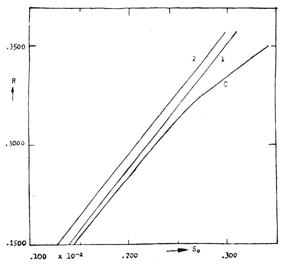
Fig. 4. Iris Image Area versus Astrophotometer Reading.
mately constant difference between calculated and observed magnitudes was found. In the next trial, Curve C was changed into Curve 1 (Fig. 4) with no sensible curvature. The constant difference between observed and calculated magnitudes was reduced. A second trial to eliminate this constant difference resulted in Curve 2. This yielded agreement in the magnitudes.
An application of the aforementioned steps results in the final corrected magnitudes shown in table 3. The calculated magnitudes are sufficiently close to the observed photoelectric magnitudes.
We can now proceed to prepare a correction table for either astrophotometer readings or magnitudes with various background emulsion densities.
The last-mentioned table is one step further than the previous one, and can be derived from it by using the calibration curve for NGC 6531 in Figure 3. This table will simplify the derivation of background corrections. The derivation of the table is based on the following facts:
1) Curve 2 of Figure 4 has no sensible curvature. Thus it can be represented by a straight line, with the equation
\[S_o \times 10^2 = 1.6 (R_o - 0.2500) + 0.126,\]
TABLE 3. Calculations of \(m_B\)
| Walker's Number | Reading | Mean Back- ground. | Density | 10-D | \(S_o\) | 110 | \(S_{i,c}\) | \(\mathcal{S}_{c}{}'\) | \[\operatorname*{Calc.}_{m_{B}}\] | Obs. \(m_B\) | \[\begin{array}{c} \text{Uncorrected} \\ m_B \end{array}\] |
|---|---|---|---|---|---|---|---|---|---|---|---|
| 56 31 56 | .3918 .3618 .3943 | .3102 .3244 .2743 | .765 .829 .605 | .172 .148 .248 | .357 .307 .361 | .852 | .203 .140 .241 | .231 .164 .271 | 10.42 12.08 9.48 | 7.52 8.65 7.42 | |
| 52 61 105 | .3006 .3970 .3390 | .2423 .3102 .2397 | .462 .765 .450 | .346 .172 .355 | .207 .366 .270 | .838 | .123 .199 .188 | .152 .228 .217 | 10.76 | 10.41 10.70 | 10.99 7.33 9.52 |
| 55 42 49 | .3508 .4098 .3261 | .2414 .3121 .2493 | .457 .774 .492 | .350 .168 .322 | .289 .387 .248 | .832 .678 | .205 .242 .168 | .234 .271 .194 | 9.50 11.34 | 11.22 | 9.07 6.85 10.01 |
| 41 111 76 97 | .2994 .2834 .3810 .3313 | .2446 .2292 .2743 .2595 | .472 .404 .506 .538 | .338 .395 .312 .260 | .215 .179 .339 .257 | .605 .688 | .106 .106 .229 .158 | .143 .135 .264 .184 | 12.80 9.64 | 10.05 11.70 7.93 9.81 | |
| 32 43 116 54 | .3505 .3894 .3058 .3640 | .2585 .2500 .2201 .3203 | .534 .496 .363 .811 | .293 .318 .434 .154 | .288 .353 .216 | .707 .682 .566 | .194 .248 .153 .145 | .222 .285 .181 .171 | 10.6 9.16 | 10.52 9.11 11.63 | 9.09 7.61 10.79 8.57 |
NOTE: Multiply Columns for \(S_o\), \(S_{i,c}\) and \(S_c\) by \(10^{-2}\)
\\'here So is the area of the iris image and Ro is the astrophotometer reading.
2) Similarly, a plot of the star image area, Sr.,, fot stars in NGC 6531 (the one in the clear area) versus the iogarithm of astrophotometer readings tbr their magnitudes, R", of the corresponding stars, yields a straight line. -fhe following table lists for example some readings rvith the corresponding star image area for stars in NGC 6531:
'fABr-D .+. Astrophotometer ReaCing R" versus image Area Sr,"
| R, | E." | |||
|---|---|---|---|---|
| 0.2600 | 0.110 x 10⁻² | |||
| .2765 | .148 , , | |||
| .2948 | .769 ,, | |||
| .3148 | 205 , t | |||
| .3496 | .2+0 ,, | |||
The straight line representing S;." as a function of log R" has the equation.
\[S_{i,c} = (1.04 \log R_c + 0.518) \times 10^{-2}\]
^9r," rn'as assumed to equal Sr,o and thus the follou'ing equation can be written:
\[S_{i,c} \times 10^2 = 1.04 \log R_c + 0.518\]
Cornbining this equation rvith the follou'ing equatit-rns:
\[S_{\epsilon} \times 10^{2} = 1.6 (R_{o} - 0.2500) + 0.126\]
\(S_{\epsilon} \times 10^{2} = 1.6 (R_{\epsilon} - 0.2500) + 0.126\)
lve get the follorving formula for the Warner and Srvasey astrophotometer:
\[R_o = \frac{R_c - 0.1712}{T} + 0.1712 - 0.625 \frac{B}{T} (1.04 \log R_c + 0.518)\] where \[T = 10^{-D}\]
\[B = 1 - 10^{-D}\]
Ro: reading on star in obscured area
R.,.- reading on star if the area rvere cleared of background densitv.
By making use of the calibration curve of Fig. 3 the corresponding magnitudes to \(R_o\) and \(R_c\) can then be obtained. Table 5 shows the results for densities from 0.08 to 0.18.
TABLE 5. Correction Table for Third Largest Diaphragm
| Uncorrected \(m_o\) | C | D | |||||
|---|---|---|---|---|---|---|---|
| \(D_o = 0.08 D_o = 0.10 D_o = 0.12 D_o = 0.14 D_o = 0.16 D_o = 0.18.\) | \(\operatorname{Corr}_m\) | \(R_c\) | |||||
| 13.93 | 13.84 | 13.76 | 13.67 | 13.58 | 13.49 | 14.21 | 0.2250 |
| 12.69 | 12.64 | 12.57 | 12.52 | 12.46 | 12.40 | 12.86 | .2500 |
| 11.66 | 11.62 | 11.57 | 11.53 | 11.48 | 11.44 | 11.81 | .2750 |
| 10.66 | 10.62 | 10.57 | 10.53 | 10.48 | 10.43 | 10.82 | .3000 |
| 9.65 | 9.59 | 9.52 | 9.50 | 9.45 | 9.40 | 9.82 | .3250 |
| 8.69 | 8.63 | 8.58 | 8.53 | 8.46 | 8.41 | 8.89 | .3500 |
| 7.72 | 7.66 | 7.58 | 7.52 | 7.45 | 7.37 | 7.96 | .3700 |
| 6.74 | 6.66 | 6.57 | 6.49 | 6.40 | 6.31 | 7.03 | .4000 |
| 5.75 | 5.64 | 5.53 | 5.45 | 5.33 | 5.21 | 6.28 | .4250 |
We should remind the reader that Curve 2 of Fig. 4 is valid only for the photographic plate containing NGC 6530 and only for the particular measurement made on it during this study. We shall now show how after such a single measuring period a good first approximation to the iris image area vs. astrophotometer reading calibration may be written once and for all which reduces trial and error labor for any plate. The principle is to transform the magnitudes and densities measured in a plate needing background correction to the magnitudes and densities of the correction table, in this case Table 5. This is summarized as follows:
- 1) Suppose an observer measured the standard sequence in a clear region of his plate. Corresponding to the same photometer readings he can obtain magnitudes which these reading would have had if measured one the plate containing NGC 6531 and 6530. These can be read from the calibration curve in Figure 4 or from the last column in Table 5. Let us call this Plot A.
- 2) Before and after measuring the plate having nebulous background, he measures the standard wedge at the numbered points used
- 3) Determine the uncorrected magnitudes of a field star by the usual photometric measurement. Call it m. From Plot A obtain the corresponding magnitude \(m_o\) of Table 5.
- 4) Use Plot B to get the density \(D_o\) from the measured background density D near the star concerned.
- 5) Then enter in Table 5, under the appropriate \(D_o\) column, the magnitude \(m_o\), and read horizontally to the corrected magnitude \(m_B\).
- 6) Re-enter on Plot A the magnitude \(m_{B_0}\) which is on the magnitude system of Table 5 and obtain the corrected magnitude m on the system for the star concerned.
There is one condition which sould be mentioned in applying the above summarized procedure, viz. The same astrophotometer comparison beam diaphragm should be used.
We should also remind the reader that any mechanical change or a change in the electronic parts may change the correction diagram considerably. Thus new tables would have to be prepared. The present diagrams, however, can be used so that very rapid approximations can be obtained for other circumstances.
If the change in Curve 2, Fig. 4, is not large, differential corrections can be applied to the tables. If electronic computers are available the programming cards of the original correction formula 5 can be made once and for all, and any change on the photometer can be followed rapidly by new tables as computed by the computer. One change in an electronic part of Warner and Swasey's astrophotometer turned out to change the curve for the iris area versus reading by about 0<sup>m</sup>.2 for the whole range of magnitudes. This proves that a change in electronic parts may give a translational shift to the curves on the correction diagram. A change in a mechanical part may well change the slope of the curves. Thus the conditions of the astrophotometer should always be checked so that any instrumental change can be followed by a new correction table. A remark may be added that the corrections for stars located in a very black part of the emulsion were observed to be more inaccurate than for those in the less black regions, because the iris had to be opened so much in measuring the densities which caused the resulting reading to be influenced by the variations in density of the emulsion.
4. ACKNOWLEDGEMENTS.
The author is much indebted to Drs. S.W. Mc Cuskey, V.M. Blanco and C.B. Stephenson for their advice. The author would like also to thank Drs. J.J. Nassau and P.P. Pesch for useful discussions during his stay in Cleveland. To Unesco and the United States A.I.D. he expresses his sincere gratitude for their scholarships.