M. Barmawi.

Department of Physics. Bandung Institute of Technology.

ICHTISAR.

Disini dibahas sarat-sarat untuk singularitas riel terdekat dari amplitudo proses2 Disini dibahas sarat-sarat untuk singularitas riel terdekat dari amplitudo proses² jang ditundjukkan oleh suatu diagram Feynman dengan satu lingkaran terutup jang umumnja menjatakan produksi dari partikel². Telah ditundjukkan, bahwa sarat Landau dan positipnja parameter Feynman jang bersangkutan tidak tjukup. Sarat selandjutnja jang masih harus dipenuhi ternjata merupakan perluasan dari sarat Karplus, Sommerfield dan Wichmann jang diketemukan untuk "fungsi tiga titik". Selandjutnja akibat sarat tambahan ini dibahas, dimana ditundjukkan pula hubungannja dengan "dugaan" (conjecture) dari Nambu dan Blankenbeckler jang ternjata umumnja tak benar. Pembahasan ini djuga dapat dipergunakan pada diagram Feynman

jang sembarang.

ABSTRACT.

The nearest real singularities of production amplitude corresponding to a single loop Feynman diagram is discussed. It is shown that Landau condition and the positiveness of the Feynman parameter is not sulfficient for the part of Landau curve to be the nearest real singularity. The additional condition is the generalized Karplus, Sommerfield and Wichmann condition, originally found in the 3-point function.

The consequences of this additional condition is discussed and related to Blankenbeckler-Nambu conjecture. The discussion is also applicable to an arbitrary Feynman diagram.

1. INTRODUCTION.

Singularities of Fevnman diagrams in general has been studied by Landau¹ and Polkinghorne and Screaton², whose results are equivalent to a certain extend. For simplicity we restrict our self to the case of singleloop diagrams. In this case the amplitude is given by (see also sec. 2)

\[V = \int_{0}^{1} \Pi dx_{i} \, \delta(1 - \Sigma_{i} x_{i}) \, D(x_{i}, p_{ij})^{-(n-2)}\]

The condition for the singularities are:

• (i)Either \(x_i = 0\)or \(\delta D/\delta x_i = 0\) with the singularities of the integrand pinching the contour of integration over \(x_i\).
• (ii) \(x_i > 0\), which is called the positiveness condition.

These will determine the nearest singularities of a single-loop diagram. In practice the difficult part is the verification of the pinching of the singularities. This is due to the multiple integration over \(x_i\) in the expression for V. For this reason in most of the study of the nearest singularities⁴ this has been neglected, hoping that it is satisfied automatically. In the present paper we are concerned with this problem, i.e. the formulation of the pinching condition and to answer the question, whether, the positiveness condition is sufficient for the part of the Landau curve to be the nearest singularity.

The present method is based on Plemelj formula⁵ and the condition for singularity is expressed geometrically. Later this condition is formulated as a set of inequalities, which corresponds to a certain region in the Landau graph. It turns out that the result is nothing, but the generalization of Karplus, Sommerfield and Wichmann condition⁶. Further it is shown that this KSW condition is equivalent to the pinching one.

In sec. 2 the idea will be explained for the case of the vertex function. An explicite example is presented which shows that the positiveness condition is not sufficient for a point on the Landau curve to be a singularity. This is also evident from the discussion. In sec. 3 we generalize the result to an arbitrary single-loop diagram with n vertices.

Our method is also applicable to any Feynman diagram, as one can see from the Chisholm expression^3,7.

2. THE VERTEX FUNCTION.

Analytic properties of the vertex function has been discussed by several authors \(^{3.8.9,10.6}\), however for later discussion it is necessary to present this in such a form that the algebra of the quadratic forms is reduced to that of corresponding matrices. Consider the vertex function associated with the process shown in fig. 1. \(m_i\) are the internal masses and \(p_{ij}\) are the four-momenta of the external particles. Using scalar fields for all the particles involved and scalar trilinear interaction on each vertices one obtaines finite expression for the vertex function. After performing symetric integration one obtain:

\[V = \int_0^1 dx_1 dx_2 dx_3 = \delta(1 - x_1 - x_2 - x_3). D^{-1} \dots (1)\]

Where D is a homogeneous quadratic form in \(x_i\):

\[D = (\Sigma_i x_i)^{-1} (\Sigma_i x_i \Sigma_i x_i m_i^2 - \Sigma_{ii} x_i x_i p_{ii}^2)\]

We can write D as a matrix product \(x^{T}(D)\) x, where \(x^{T} = (x_1, x_2, x_3)\) and the matrix (D) is:

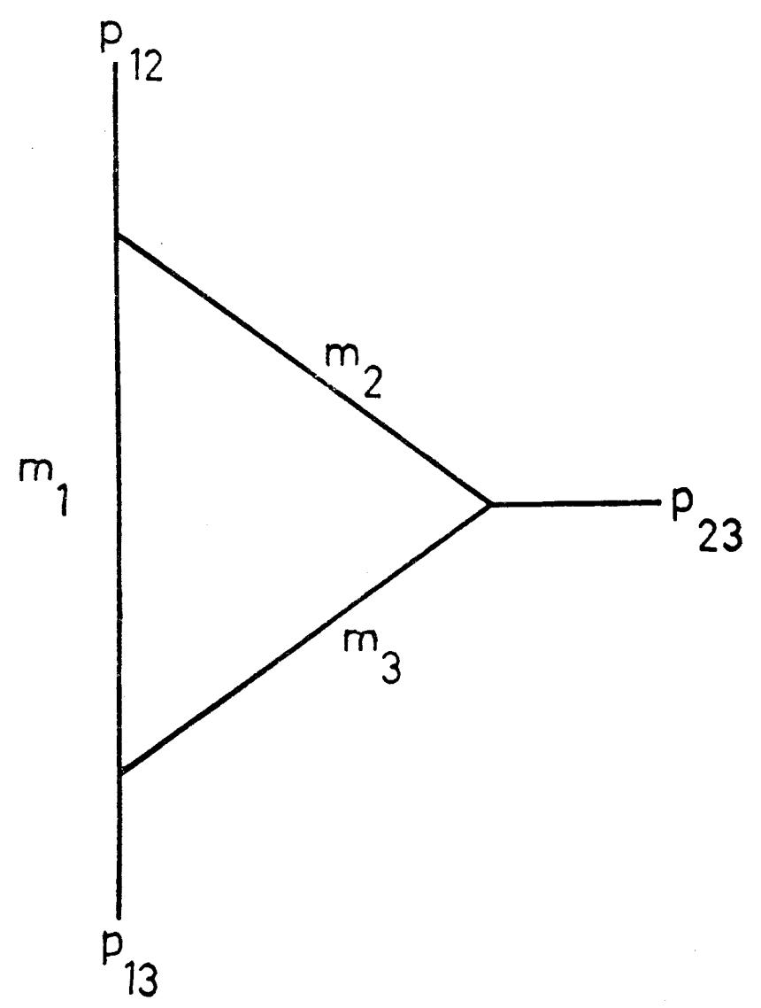
Fig. 1. The vertex function.

\[\begin{pmatrix} 2m_1^2 & m_1^2 + m_2^2 - p_{12}^2 & m_1^2 + m_3^2 - p_{13}^2 \\ m_1^2 + m_2^2 - p_{12}^2 & 2m_2^2 & m_2^2 + m_3^2 - p_{23}^2 \\ m_1^2 + m_2^2 - p_{13}^2 & m_2^2 + m_3^2 - p_{23}^2 & 2m_3^2 \end{pmatrix}\]

If we carry out the integration over \(x_3\) the vertex function becomes

\[V = \int_0^1 dx_1 \int_0^{1-x_1} dx_2 D_s^{-1}\]

The matrix of \(D_s\) is most easily obtained from (D) by considering the substitution \(x_3 = 1 - x_1 - x_2\) as a linear transformation from \((x_1, x_2, 1)\). For later discussion it is important to note that the determinant of this transformation is unity. All these can be generalized to single-loop diagrams with the number of external masses greater than 3.

A dispersion relation is essentially a Cauchy integral representation⁵. Originally it is known the case, where we have only the normal threshold, which comes from the lower limit of the mass spectrum so that one usually integrate over a part of the real axis. If we have a cut which goes off the real axis we have to generalize the contour to the cut. If the condition for the existence of the Cauchy integral representation is satisfied then the dispersion relation in nothing but the Plemelj formula⁵:

\[\frac{1}{2}(V^{+}+V^{-}) = (1/\pi) \int_{L} \frac{A(p_{1},\sigma)}{t-\sigma} \cdot d\sigma\] \[A(p,\sigma) = \frac{1}{2i}(V^{+}-V^{-})\] where \(p_1 = (p_{12}^2, p_{13}^2)\) and \(+t = p_{23}^2\) is the momentum transfer. Here t is not retricted do the regular points of V. The superscript \(\pm\) denotes the limiting process from 2 opposite sides of the contour, when t is on L. Let us make 2 assumptions:

• 1) The existence of such an integral representation for V
• 2) L is a part of the real axis. The second assumption, is the same as assuming that the singularities are real, however we do not assume that L starts from any particular point of the real axis. Later on we will discuss these assumptions. By these assumptions one can calculate the absorptive part A using the identity: \((a io)^{-1} (a + io)^{-1} = 2\pi i \delta(a)\),

\[A(p,\sigma) = \int_{0}^{1} dx_{1} \cdot \int_{0}^{1-x_{1}} dx_{2} \cdot \delta(D_{s}) \cdot \dots (2)\]

Let us associate a geometric picture to the computation of this integral. The boundary of integration of integral (2) is an equilateral triangle in the \(x_1\), \(x_2\) plane. D=0 is a conic. The non-zero contribution to the integral

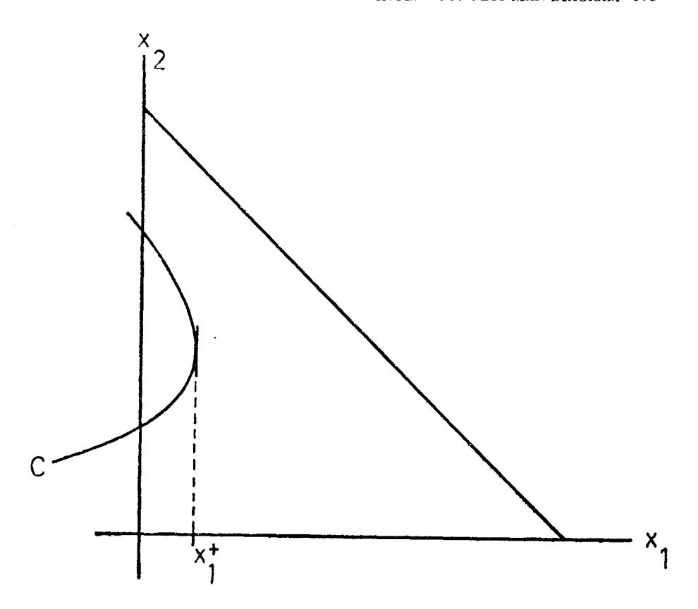
Fig. 2. The equilateral triangle is the boundary of integration of (2). C is the curve D=0. 0 and \(x_1^+\) are the boundary of integration for the absorptive part of the vertex function.

comes from the zeros of D, hence "A=0 only if there is a part of the conic which lies inside the triangle T"—note that the shape and the position of the conic depends upon \((p_1, \sigma)\). It is obvious that at the threshold of V the conic start to enter T. There are only two ways for \(D_s=0\) to enter into T, i.e. when it touches the boundary of T or suddenly appears as a point-ellips inside T.

Therefore:

• (i) At the normal threshold of V, the conic \(D_s = 0\) is tangent to one of the sides of T.
• (ii) At the anomalous threshold, the conic \(D_s = 0\) suddenly appears in T as point-ellips.

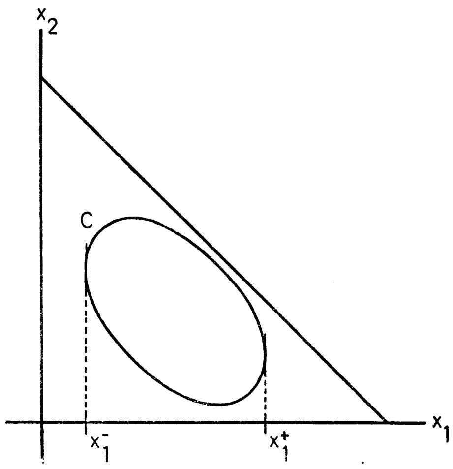
Fig. 2 a. The equilateral triangle is the boundary of integration of (2). C is the curve D = 0. \(x_1^{\pm}\) are the boundary of integration for the absorptive part of the vertex function.

(ii) comes from the fact that as the ellips grows, it touches the side of the triangle from inside at the normal threshold. These lead to the same eqs. of Polkinghorne — Screaton (PS) — condition (i) of sec. 1—— that is: (i) is equivalent to

\[x_1=0\]; \(\frac{\delta D}{\delta x_j}=0\) (\(j=2,3\)) and (ii) with \(\frac{\delta D}{\delta x_i}=0\) (\(i=1,2,3\)), and constitute a homogeneous linear eqs. for \(x_j\), whose solution with \(x_1+x_2+x_3=1\) gives the coordinates of the point of tangency and of the point-elips respectively. The equation of singularities comes from the requirement that these eqs. has a non-trivial solutions, that is the 2 by 2 main-minor of det. (D) in the normal case, and the determinant of (D) itself in the anomalcus case, is equal to zero. The requirement that the tangent point or the point-ellips to belong to the closed region T is essentially the positiveness condition (ii) of sec. 1. We have reproduced the equation of the singularities and the positiveness condition in our picture. However (ii) is more than that, it requires that D=0 is a point-ellips. This does not follow from det. (D) = 0. The last equation says only that D = 0is degenerate. Since we have one centre of symmetry the posibility of being a pair of intersecting lines is not excluded. The point-ellips condition will be formulated by saying that D=0 will not intersect \(x_i=0\) (i=1,2). This leads to the 2 by 2 main-miror of det. (D) must be positive. This is essentially the same as Karplus-Sommerfield-Wichmann condition⁶, which is obtained and expressed in a different way. To illustrate the situation we take as an example the form factors, where \(p_{12}^2 = p_{13}^2 = z\). We restrict ourself to real internal masses. In this case \(det.(D) = -t \{m^2t - z\}\)(4m - z) = 0 all internal masses being equal to m. The curve of singularities, the Landau curve, in the real. (z, t) plane is shown in fig. 3. \(z=t=4m^2\) are the normal thresholds. In the interior of the square \(0 < 4m^2\), \(0 < t < 4m^2\), the main-minors are positive. Shaded region is the region of positive Feynman parameters \(x_i\). We conclude from the above discussion that only the part of det. (D) = 0 which lies in the intersection of the two regions will give the anomalous singularity in the physical sheet. This is wellkown. However what happens if \(z > 4 m^2\)? If this inequality is satisfied then D=0 always cut \(x_3=1-x_1-x_2=0\) and \(x_2=0\) at two points on each. However now the validity of (2) is doubtful, since V is no longer single-valued, because we are on the cut in z complex plane. (Cf. Plemelj formula for t on the cut). Therefore nothing can be said at this point. Oehne has shown⁸, by analytic continuation of the differentiated form of V, that the singularity disappears from the physical sheet. This shows that the positiveness condition is not sufficient. The singularity is the nearest since we approach it from the physical region, which is regular³.

Let us go back to the calculation of the absorptive part A in (2). The result of \(x_2\) integration is \(2.R_2\) \((D_s^{\frac{1}{2}})\), where \(R_2(D_s)\) is the discriminant of \(D_s\) with respect to the parameter \(x_2\). Then

\[A(z,\sigma) = \int_{-x_1^{-}}^{x_1^{+}} dx_1 \cdot 2R_2(D_s)^{\frac{1}{2}}, \quad \text{for } \sigma_a < \sigma < \frac{4}{7}m^2\]

\(\sigma_a =\) anomalous threshold.

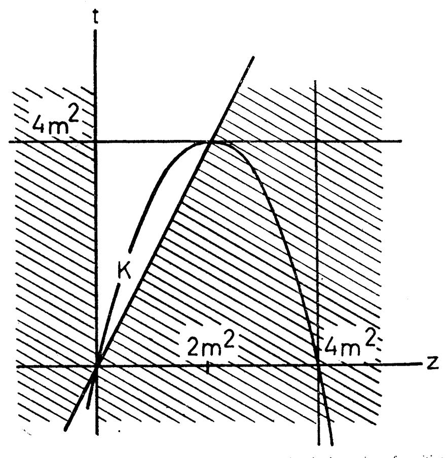
Fig. 3. K is the curve det (D) = 0. Shaded region is the region of positive Feynman parameters.

and \[A(z, \sigma) = \int_{0}^{x_{1}^{-1}} x_{1} dx_{1} \cdot 2R_{2}(D_{s})^{\frac{1}{2}},\] for \(\sigma > 4m^{2}\)

if \(2m^2 < z < 4m^2\). The boundaries of the first integral is between the two vertical tangents to the conic \(D_s = 0\), while the second is between the \(x_2\) axis and the vertical tangent inside T. Note that in the first case the ellips is inside T. If \(z > 4m^2\) then the integral is only equal to the second one. We see that the effect of the normal threshold in the anomalous case disappears, as first observed by Blankanheckler and Nambu ¹⁰. This is clear in our picture since in the anomalous case the conic touches the \(x_2\) axis from inside, while in the normal case it is from outside of T.

This section will be closed with some remarks. Firstly, the procedure leads to the correct physical sheet is clear, since we have used the vertex function defined by the definite real integral (1) over the Feynman parameters^3,8, in contrast to PS treatment where it is extended to the complex one. Consequently instead of the pinching we have the point-ellips condition. Second, the assumption that the singularities are real is not serious, since we know the Landau curve. By restricting some parameters to a certain range this can be satisfied. Thirdly, the assumption about the existence of the Cauchy integral representation is reasonable. The condition for this is that the absorptive part satisfies the Hölder condition⁵. Estimates of the behaviour of V near the singularities ^1,2,11 shows, that indeed the H condition is satisfied.

3. THE SINGLE-LOOP FEYNMAN DIAGRAM.

The amplitude of a single-loop diagram with n external particles, which corresponds to production process, is

\[V = \int_{0}^{1} \Pi_{i} dx_{i} \quad \delta(1 - \Sigma_{i}). D^{-(n-2)} \quad ...\] (3)

where the index i runs from 1 to n. D is the same as in the vertex function except that now the range of the index is extended up to n. The trouble in generalizing the previous result is, that now the power of D is \(-(n-2) \neq -1\), so that we cannot use the method of sec. 2. For this reason we construct a new function: F defined in the same way as V with a change in the power of D; instead of -(n-2) we take -1. V is then related to F by the following differential operation with respect to the internal masses:

\[V = (\Sigma \delta / \delta m_i^2)^{n-3} F.\]

The analytic properties of F and V will be the same, although the types of singularities might be different⁹. The corresponding integral to (2) for the absorptive part of F is now over an n-1 dimensional equilateral "Tetrahydron" \(T_{n-1}\) in n dimensional Eucledian space bounded by the hyperplanes \(x_i = 0\) \((i = 1, 2, \ldots, n)\), where \(x_n = 1 - (x_1 + x_2) + \ldots + x_{n-1}\).

Using the classification of Tarski¹¹ we can formulate the condition for the nearest real singularities of a single-loop diagram as:

"At the \(C^k\) singularity of a single-loop Feynman diagram with n external masses:

• (i) for k < n-1 the hypersurfase D-0 is tangent to a k dimensional plane \(x_i = 0\) (for some n-k Feynman parameters) as a boundary of \(T_{n-1}\) at one-point.
• (ii) for k = n 1 D = 0 is a point-hyperellipsoid inside \(T_{n-1}\). Note that for a higher dimensional quardratic surface it is possible that a hyperplane is tangent to it with a lower dimensional plane in common—We will discuss only (ii) since (i) is essentially the same problem in a lower dimensional space.

As before the conditions lead to the PS equation of singularities and the positiveness condition. Let us find the point-hyperellipsoid condition more explicity. Here we also try to find the intersection with some \(x_i = 0\). The intersection is given by the equation \(D(x_i \neq i, x_i = 0) = 0\).

For this to have no real points, this D must be either negative or positive definite. If the internal masses are real, the first possibility is excluded. A theorem on quadratic forms¹² states that a necessary and sufficient condition for a hermitian quadratic for to be positive definits is, that the determinant of its matrix and all its main-minore are positive. Since the determinant of \((D_s)\) and all its main-minors is the same as that of (D) (cf. remark in the begining of sec. 2.) it follows that: "The condition for the nearest real singularities of type \(C^k\) whose equation is det. \((D)_k = 0\) is that all its main-minors are positive." in addition to the positiveness condition. \((D_k)\) is the "main-minors" of the matrix (D) which is k by k. An immidiate consequence of this is that the nearest real singularity of a single-loop diagram is located in a finite region.

Since the tangency of the quadratic surface to a k-1 dimensional plane on the boundary of \(T_{n-1}\) can only occur after it touches a k dimensional plane, it follows that: "The nearest real singularity of type \(C^{k-1}\) is farther than that of type \(C^k\) with respect to the origin." In the \(C^k\) singularity, the \(C^i\) one (i < k) does not "affect" the absorptive part of presence of F. This can be easily visualized in the case of the four-point function. Hence F will certainly satisfy the conjecture of Blankenbeckler and Nambu¹⁰, however it is not necessary true for \(\Gamma\). This is clearly shown in an example given by Ochme in the case of vertex function.

Finally we would like to relate the pinching with the point-hyperellipsoid condition. If we are off the Landau curve in the physical region then D is positive definite. Since the matrix (D) is the roots of hermitian D\((x_i)\) in each Feynman parameter are complex conjugate one to another, they lie on the opposite sides of the real axis in the \(x_i\) complex plane. As we let the point approach the Landau curve these singularities pinch the real axis.

4. ACKNOWLEDGEMENT.

The auther would like to thank Professor Oehme for guidance to the subject during the former residence at the University of Chicago and Professor Eden for explaining the situation of the positiveness and pinching condition, which leads to writing the present paper.

5. REFERENCES.

• 1) L.D. Landau, Nuclear Physics, 13, 181 (1959)
• 2) J.C. Polkinghorne and G.R. Screaton, Nuovo Cimento X, 15, 289 and 925 (1960). This will be referred as PS.
• 3) R.J. Eden, Phys. Rev. 119, 1763 (1960); 120, 1514 (1960) For the physical significance of the singularities and a thorough review we refer to R.J. Eden, Physics Department Technical Report No. 211 (1961) Univ. of Maryland.
• 4) see for example: L.B. Okun and A.P. Rudik, Nuclear Physics 14, 261, (1960) Report presented by A.P. Rudik in "Proceedings of 1960 Annual International Conference on High Emergy Physics at Rochester" (Interscience, 1960).
• 5) N.I. Muskehlishvili: "Singular Integral Equation" (1953).
• 6) R. Karplus, C.M. Sommerfield and E.H. Wichmann, Phys. Rev. 111, 1187 (1958).
• 7) R. Chisholm, Proc. Camb. Phil. Soc. 48, 300 (1952).
• 8) R. Oehme, Phys. Rev. 111, 1430 (1958).
• 9) R. Oehme, Nuovo Cimento X, 13, 779, (1959).
• 10) R. Blankenbeckler and Y. Nambu, Nuovo Cimento, 18, 595 (1960).
• 11) J. Tarski, Journal of Math. Phys. 1, 154 (1960).
• 12) Handb. d. Physik II, p.62, Satz 28.