

1. Introduction
The effect of body forces, i.e. not surface forces, on the contact angle formed by a solid, a liquid and a gas is of interest lately. In problems leading to burn out, which are important in nuclear reactors and the cooling of rocket nozzles, one deals a lot with the so-called "dynamic" contact angle associated with the formation of dry-spots.
A more detailed insight into the question of the contact angle variation with body forces, can be obtained, although for a more simple problem, using a microscopic approach. This approach uses a simple intermolecular potential along the method proposed by Flachsbart and Anliker (1). The problem treated here is an extension of their work by including the effect of the centrifugal force, besides the gravity force, to affect the contact angle. It will be shown, that the contact angle is not affected by the accounted body forces on a zeroth order basis.
2. The problem and assumptions
The configuration considered here is shown in Figure 1, where r, 0 and z are variables of a cylindrical coordinate system that is applied. A circular pan containing liquid is rotated, such that a dry-spot occurs in the center, while the liquid is thrown to the peripheral wall of the pan as shown in the constant \(\theta\) cross-sectional view of Figure 1. The volume of the liquid is constant
*) Department of Mechanical Engineering Institute of Technology Bandung.
Figure I 'l he configuration considered: solicl body rotltion of a liguid in a rotating Ptn.
and the liquid is assumed to tre in a solid bo<ly rotation at a constant anglrlar velocity o. The liquid is assumed to be distributed symnletricrlly around the axis of rotation, i.e. the z-axis and tirrthermore, assunle b<< a.
The following assurnptions are made fbr the internrolecular model:
l. The intenrrolecular attraction potential is assumed to take the same form, both for an inter-species and a diff'ering spccies intcraction of nrolecules, except for the constant K1,11 :
\[P_3 = -\frac{K_{I,II}}{r^6} \tag{1}\]
uhcre K1,11 is a constant applicable for the interaction between mclecules of species I anrl II (for an inter-species interaction it becomes Kr,r), r the intermolecular distance between two molecules, ancl P., defincs the three dimensional attraction potential bctween two nrolecules.
2. The force defined by thc potential as in EqLration (l) decreases rapidly as the intermolcculitr distance, r, increases. To sirnplity the calctrlation of the potential of a molecule clue to the interaction of other neighboring molecules, it is assumed, that beyond a certain distance, called the cut of distance, A, the lbrce of inleraction is neglected. This assurnption is reasonable, because the inter:action potential is a function of the inverse of the sixth power of the intermolecular distance. Furthermore, in evah.rating the potential of a molecule, the surrottndiug molecules may be assuned to be continuously distributed.
Consider the molecule located at the center of the spheres drawn in Figure 2. tf 8r is taken to be half of the average distance betrveen two molscules of type I, then all the molecules outside this distance may be treated as
Figure 2 The volume of integration for the potential of a species molecule due to surrounding molecules.
continuously distributed. Let \(n_1\) denote the molecular density of species I. Then the potential of a molecule can be estimated by
\[P_{\text{total}} = -n_{\text{I}} \iiint_{V} \frac{K_{\text{I,I}}}{r^{6}} dV\] (2)
where the integration is carried out over the volume, V, which is between the spheres of radius \(\delta_1\) and \(\Delta\).
By assumptions 1 and 2, the total potential of all the molecules of the constant volume rotating liquid given in the configuration of Figure 1, can be estimated. The calculation procedure is as follows. A cross-sectional view \((\theta = \text{constant})\) of the configuration considered here is divided into four rings, as shown in Figure 3, according to the type of interaction. The cross-sectional
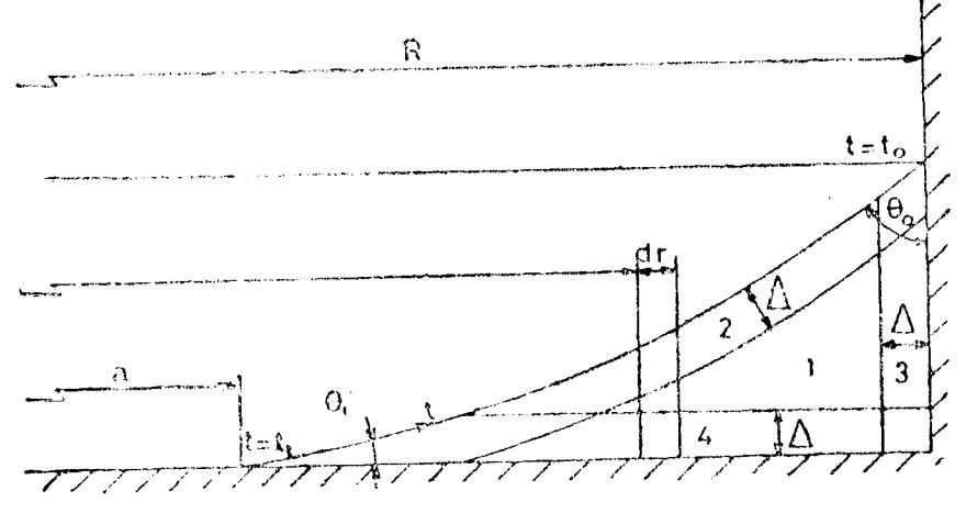
Figure 3 Division into rings.
view of these rings is denoted by 1, 2, 3 and 4 respectively. It can be directly seen, that a liquid molecule in 1 interacts solely with liquid molecules. Furthermore, it is obvious that a liquid molecule of ring 2 interacts with both gas and liquid molecules.
Therefore, the potential of a liquid molecule located inside the ring, which cross-sectional area is 1, becomes:
\[U_{LL} = \int_{r=\delta_{L}}^{\Delta} \int_{0=0}^{\pi} \int_{\varphi=0}^{2\pi} \frac{K_{LL}}{r^{6}} n_{L} r^{2}(\sin \theta) d\theta d\varphi dr\] \[= \frac{4}{3} \pi n_{L} K_{LL} \left(\frac{1}{\Delta^{3}} - \frac{1}{\delta_{L}^{3}}\right)\] (3)
where the subscript L is used to indicate the liquid.
Throughout the analysis, it is further assumed that \(\delta_{\rm I} << \triangle\), such that terms of order \(\frac{1}{\Delta^3}\) can be neglected compared to \(\frac{1}{\delta_{\rm L}}\). This assumption is consistent in the accuracy of the analysis as illustrated by the overlapping regions of cross-sectional areas 2 & 3, 2 & 4 and 3 & 4.
Consider a liquid molecule, which may be located in the rings: with cross-sectional area 2, 3 or 4, and located at a distance y from the interface involved. In Figure 3 one can see, that area 2 involves a liquid-gas interface, while areas 3 and 4 both involve liquid-solid interfaces. Now, for a molecule of this type, i.e. located at a distance y from any of the mentioned interfaces associated with areas 2, 3 or 4, the potential due to intermolecular interaction is calculated by (see figure 4)
Figure 4 Treatment of a liquid molecule near an interface.
\[\begin{split} U_{Lj} = & -n_L \ K_{LL} \int\limits_{r=0}^{y} \int\limits_{\theta=0}^{\pi} \frac{2\pi}{r^6} \, d\theta \, d\phi \, dr \\ & r = \delta_L \int\limits_{\theta=0}^{t} \int\limits_{\phi=0}^{r^2 \sin \theta} \, d\theta \, d\phi \, dr \\ + \int\limits_{r=y}^{\Delta} \left[ -\int\limits_{\theta=0}^{t} \frac{n_j \ K_{Lj}}{r^6} \int\limits_{\phi=0}^{r^2 \sin \theta} r^2 \sin \theta \, d\phi \, d\theta \right] \\ - \int\limits_{\theta=cos^{-1}}^{\pi} \frac{n_L \ K_{LL}}{r^2} \int\limits_{\phi=0}^{2\pi} r^2 \sin \theta \, d\phi \, d\theta \, d\theta \, d\theta \end{split}\] or,
\[U_{Lj} = \pi \, n_j \, K_{Lj} \left( \frac{2}{3\Delta^2} - \frac{y}{2\Delta^4} - \frac{1}{6y^3} \right)\] \[+ \pi \, n_L \, K_{LL} \left( \frac{y}{2\Delta^4} + \frac{2}{3\Delta^2} - \frac{4}{3\delta_L^2} + \frac{1}{6y^3} \right)\] (4)
Here the subscript j is used for any of the species involved in the interface interaction of areas 2, 3 or 4, except to indicate the liquid molecule.
Consider a volume element with the sides \(rd\phi\), \(\Delta\) and a unit length along the 0-direction located in any of the rings 2, 3 or 4. For this volume element the potential is approximated by
\[\overline{U}_{Lj} = \left( \int_{y=\delta_L}^{\Delta} n_L U_{Lj} \, dy \right) r d\phi,\] which upon using (4) becomes
\[\begin{split} \overline{U}_{Lj} &= \left[ \pi n_L \; n_j \; K_{Lj} \left( \frac{1}{2\Delta^2} - \frac{2\delta_L}{3\Delta^2} + \frac{\delta_L^2}{4\Delta^2} - \frac{1}{12\delta_L^2} \right) \right. \\ &+ \left. \pi n^2_L \; K_{LL} \left( -\frac{\delta_L^2}{4\Delta^4} - \frac{2\delta_L}{3\Delta^3} + \frac{10}{12\Delta^2} + \frac{17}{12\delta_L^2} - \frac{4\Delta}{3\delta_L^3} \right) \right] r d\phi \quad (5) \end{split}\]
Defining
\[\begin{split} \overline{U}_{Lj}^* &= \pi n_L \ n_j \ K_{Lj} \left( \frac{1}{2\Delta^2} - \frac{2\delta_L}{3\Delta^2} + \frac{\delta_L^2}{4^2\Delta} - \frac{1}{12\delta_L^2} \right) \\ &+ \pi n_L^2 \ K_{LL} \left( -\frac{\delta_L^2}{4\Delta^4} - \frac{2\delta_L}{3\Delta^3} + \frac{10}{12\Delta^2} + \frac{17}{12\delta_L^2} - \frac{4\Delta}{3\delta_L^2} \right) \end{split}\]
we can write (5) as
\[\overline{U}_{\mathrm{Lj}} = \overline{U}_{\mathrm{Lj}}^* \; r d \phi\] and observe, that \(\overline{U}_{Lj}^{\,\star}\) is a function of the microscopic constants \(\Delta,\,\delta_L,\,n_L,\)\(n_i, K_{Li}, K_{LL}\)only.
The total intermolecular attraction potential
Let the liquid-gas interface be represented by z = f(r), which in parametric form can be written as z = f(r[t]), where t is a curve parameter, such that (see figure 3), at \[r = (R - a)\], \(f[r(t)] = 0\) and \(t = t_1\)
and at \(r = R\), \(f[r(t)] = b\) and \(t = t_0\).
Using the previously given parametric representation of the interface and (3), the total potential of the intermolecular attraction of all the molecules in the ring with cross-sectional area 1 is calculated. The result is
\[U_{RL}^{(1)} = 2\pi n_{L} U_{RL} \left[ \int_{t_{1}}^{t_{0}} fr\dot{r} dt - \Delta \left( \int_{t_{1}}^{t_{0}} r(\dot{r}^{2} + \dot{f}^{2}) \frac{1}{2} dt + \int_{t_{1}}^{t_{0}} r\dot{r} dt + \int_{t_{1}}^{t_{0}} R\dot{f} dt \right) \right]\] \[(6)\] where the superscript (1) denotes the ring having cross-sectional area 1. For the rings with cross-sectional areas 2, 3 and 4, the total intermolecular potentials are calculated from (5) and are, respectively,
\[U_{LG}^{(2)} = 2\pi \, \overline{U}_{LG}^* \int_{t_1}^{t_0} r \, (\dot{r}^2 + \dot{f}^2)^{\frac{1}{2}} \, dt\] (7)
\[U_{LG}^{(2)} = 2\pi \, \overline{U}_{LG}^{*} \int_{t_{1}}^{t_{0}} r \, (\dot{r}^{2} + \dot{f}^{2}) \dot{t} \, dt\] \[U_{LS}^{(3)} = 2\pi \, \overline{U}_{LS}^{*} \int_{t_{1}}^{t_{0}} R \dot{f} \, dt\] \[U_{LS}^{(4)} = 2\pi \, \overline{U}_{LS}^{*} \int_{t_{1}}^{t_{0}} r \dot{r} \, dt\] \[(9)\]
\[U_{LS}^{(4)} = 2\pi \ \overline{U}_{LS}^* \int_{t_1}^{t_0} rr \, dt\] (9)
Here, the superscripts (2), (3) and (4) denote respectively, rings with crosssectional areas (2), (3) and (4). Hence, the total potential due to the intermolecular attraction is
\[U_{TIA} = U_{LL} + U_{LG} + U_{LS} + U_{LS}\] (10)
4. The potentials due to the accounted body forces
As was mentioned previously, two types of body forces are accounted here, namely gravity and centrifugal forces.
The conservative potential due to gravity for the configuration considered here is given by
\[U_{LGr} = \frac{2\pi \rho g}{2} \int_{t_1}^{t_0} f^2 r \dot{r} dt\] (11)
while the potential associated with the centrifugal force can be expressed as
\[U_{L}\omega = \frac{2\pi \rho \omega^{2}}{2} \int_{t_{1}}^{t_{0}} r^{3} f \dot{r} dt\] (12)
5. The stationary condition
For an equilibrium liquid-gas interface to prevail then the total potential of the system considered here must reach some kind of a stationary condition, which with less rigour can be associated with a minimum potential. It is to be recalled that the problem posseses one constraint, i.e. the constancy of the volume of the liquid. Thus the problem is essentially a variational problem, with one constraint. Let the Lagrange multiplier be denoted by \(\lambda\). The volume of the liquid is calculated to be
\[V = 2\pi \int_{t_1}^{t_0} fr\dot{t} dt \tag{13}\]
Hence, the variational problem consists of minimizing the functional
\[T = U_{TI\Lambda} + U_{LGr} + U_{L}\omega - \lambda V \tag{14}\] which upon substituting (6), (7), (8), (9), (11), (12) and (13) becomes
\[T = \int_{t_1}^{t_0} F(r, \dot{r}, f, \dot{f}, t) dt\] (15)
where
\[F(\mathbf{r}, \dot{\mathbf{r}}, \dot{\mathbf{f}}, \dot{\mathbf{f}}, t) = (\overline{U}_{LG}^* - \Delta U_{LL} n_L) \mathbf{r} (\dot{\mathbf{r}}^2 + \dot{\mathbf{f}}^2) \frac{1}{2}\] \[+ (\overline{U}_{LS}^* - \Delta U_{LL} n_L) \mathbf{R} \dot{\mathbf{f}} + (\overline{U}_{LS}^* - \Delta U_{LL} n_L) \mathbf{r} \dot{\mathbf{r}}\] \[+ U_{LL} n_L \dot{\mathbf{f}} \dot{\mathbf{r}} \mathbf{r} + \frac{\rho g}{2} f^2 \mathbf{r} \dot{\mathbf{r}} + \frac{\rho \omega^2}{2} \mathbf{r}^2 \dot{\mathbf{f}} \dot{\mathbf{r}} - \lambda \dot{\mathbf{f}} \dot{\mathbf{r}} \dot{\mathbf{r}}\] (16)
For a stationary condition to prevail then
\[\frac{\mathrm{dT}}{\mathrm{dt}} = 0\] or
\[\int\limits_{t_1}^{t_0} \dot{f} \left(F_r - \frac{\mathrm{d}F_{\dot{r}}}{\mathrm{d}t}\right) \, \mathrm{d}t + \int\limits_{t_1}^{t_0} \dot{f} \left(F_f - \frac{\mathrm{d}F_{\dot{f}}}{\mathrm{d}t}\right) \, \mathrm{d}t + \left[ \, F_{\,\dot{r}} \dot{r} + F_{\dot{f}} \, \dot{f} \, \right]_{t_1}^{t_0} = 0\] which leads to
\[\left(F_{r} - \frac{dF_{r}}{dt}\right) = 0\] (17)
\[\left(F_{f} - \frac{dF_{f}^{*}}{dt}\right) = 0\] (18)
with the following transversality conditions
\[(F_{\mathbf{i}}\dot{\mathbf{r}} + F_{\mathbf{f}}\dot{\mathbf{f}})\Big|_{\mathbf{t} = \mathbf{t_1}} = 0 \tag{19}\]
\[(F_{\dot{\mathbf{r}}}\dot{\mathbf{r}} + F_{\dot{\mathbf{f}}}\dot{\mathbf{f}})\Big|_{\mathbf{t} = \mathbf{r_0}} = 0 \tag{20}\]
Here, \[F_r \equiv \frac{\partial F}{\partial r}\], \(F_r = \frac{\partial F}{\partial r}\) etc
The assumption, that the liquid is distributed symmetrically around the axis of the solid body rotation allows the discussion of the surfaces along which the triple interaction curves (i.e. curves, along which the solid, the liquid and the gas interact) move in the process of reaching the stationary condition, in terms of curves. Denote the curves upon which the triple points \(t=t_1\) and \(t=t_0\) (of the cross-sectional view) move by the functions, see reference (2),
\[\vec{f_1} = \vec{\phi_1} (\tau)\] \(\vec{f_1} = \vec{\phi_1} (\tau)\)
and
\[\overline{\frac{r_0}{f_0}} = \overline{\phi_0} \ (\tau) \ )\] \[\overline{f_0} = \overline{\psi_0} \ (\tau) \ )\]
This is the problem of Bolza, see references (1) and (2). The movements of the edge points are then regulated by
\[\overline{r_1}' = \text{arbitrary}\] (21) \(\overline{f_1}' = 0\)
and
\[\overline{\overline{r_0}}' = 0\] \[\overline{\overline{r_0}}' = \text{arbitrary}\] (22)
because of physical reasons, i.e. points \(t = t_1\) and \(t = t_0\) move along the solid surface if no breakdowns occur. Note that the primes in equations (20) and (21) denote differentiation with respect to time, \(\tau\).
The stationary conditions (17) and (18) are not independent, see for example reference (1) for a detailed discussion. For the purpose of this paper stationary condition (17) will be used, because both (17) and (18) would give the same final result. Calculation of the required derivatives from (16) and substituting then in (17) would result in the following equation
\[(\overline{U}_{LG}^{*} - \Delta U_{LL} \, n_{L}) \left( \frac{\dot{f} \, \dot{r} - \dot{r} \, \dot{f}}{(\dot{t}^{2} + \dot{f}^{2})^{3/2}} - \frac{1}{r} \, \frac{(\dot{f}/\dot{r})}{[1 + (\dot{f}/\dot{r})^{2}]^{1/2}} \right) + U_{LL} \, n_{L} + \frac{\rho \omega^{2}}{2} \, r^{2} \, \frac{\dot{f}}{\dot{f}} + \rho g f - \lambda = 0\] (23)
which esentially is the surface tension equation in the microscopic form. For a comparison the classical surface tension equation is written here
\[\gamma \left(\frac{1}{R_1} + \frac{1}{R_2}\right) + (\rho - p_0) + \rho g f = 0\] (24)
where \(\gamma\) is the surface tension, \(\left(\frac{1}{R_1} + \frac{1}{R_2}\right)\) the principal curvature of the interface, \((p - p_0)\) the interface pressure difference and f the shape of the interface.
Upon comparing (23) with (24), the following correspondence is found
\[\frac{1}{R_1} + \frac{1}{R_2} = \frac{\dot{f}\ddot{r} - \dot{r}\dot{f}}{(\dot{r}^2 + \dot{f}^2)^{3/2}} - \frac{1}{r} \frac{(\dot{f}/\dot{r})}{[1 + (\dot{f}/\dot{r})^2]^{1/2}}\] \[\rho gf = \rho gf\]
Therefore.
\[\gamma = (\overline{\mathbf{U}}_{LG}^* - \Delta \mathbf{U}_{LL} \mathbf{n}_{L}) \tag{25}\]
\[p - p_0 = U_{LL} n_L + \frac{\rho \omega^2}{2} r^2 \frac{f}{f} - \lambda\] (26)
The transversality condition (19) combined with (21) gives the stationary condition at the triple point 1 (see figure 3),
\[\overline{r_{1}'} \left[ \frac{(\overline{U}_{LG}^{*} - \Delta U_{LL} n_{L})}{(\hat{r}^{2} + \hat{f}^{2})^{1/2}} + (\overline{U}_{LS}^{*} - \Delta U_{LL} n_{L}) + (U_{LL} n_{L} + \frac{\rho g}{2} f + \frac{f\omega^{2}}{2} r^{2} - \lambda) \right]_{t=t_{1}} = 0\] (27)
Note that at the triple point 1,
\[f \bigg|_{t = t_1} = 0 \quad \text{and} \quad \frac{\dot{f}}{\dot{x}} \bigg|_{t = t_1} = \tan \theta_1 \tag{28}\]
Combining (26) and (27) and working out the algebra result in the expression for the contact angle at the triple point 1,
\[\theta_1 = \sec^{-1} \left( \frac{(\Delta U_{LL} \ n_L - \overline{U}_{LG}^*)}{\overline{U}_{LS} - \Delta U_{LL} \ n_L} \right)\] (29)
Using a similar way, the transversality condition (20) when combined with (22) and furthermore noting, that \(\overline{r_0}' \Big|_{t=t_0} = 0\)
and \(\frac{\dot{f}}{\dot{x}}\Big|_{t=t_0} = \tan\left(\frac{\pi}{2} - \theta_0\right)\) one gets the expression for the contact angle at the triple point 0,
\[\theta_0 = \pi - \sin^{-1} \left( \frac{(\overline{\mathbf{U}}_{LS}^* - \Delta \mathbf{U}_{LL} \cdot \mathbf{n}_L)}{\Delta \mathbf{U}_{LL} \cdot \mathbf{n}_L - \overline{\mathbf{U}}_{LG}^*} \right)\](30)
6. Conclusions
The following conclusions are found for the simple problem considered here:
- 1. The surface tension between the liquid and the gas is neither affected by the accounted body forces nor by the shape of the interface. The surface tension is a function of the interacting species at the interface. This result can easily be deduced from (25).
- 2. The interface pressure difference, besides dependent on the liquid molecular properties, is found to depend on the interface shape, see equation (26). The interaction between the pressure and the interface is demonstrated. For example, the higher the angular velocity ω, the higher the interface pressure would be.
- 3. The contact angles \(\theta_1\) and \(\theta_0\), see respectively equations (29) and (30), depend only on the microscopic molecular properties of the species involved in forming the angles and for the order of approximations made here, they are neither dependent on the accounted body forces nor the interface shape.
- 4. The problem considered here clearly demonstrated the capabilities and limitations of mathematical problem specification and solution and is intended as a promotion of mathematical modeling of physical problems at the Institut Teknologi Bandung.