

I. HISTORICAL BACKGROUND
The low-speed wind-tunnel at ITB was built as a closed, single r,i:turn type and powered by an automotive engine. The automotive englne drives a generator, which supplles electricity to a direct current electric motor. The electric motor drives the four bladed propeller type fan.
The lnitial design of the lori-speed wind-tunnel at ITB was actually started in 1959 under the dlrection of the late Air Marshal Nurtanio (the director of what is now LIPNUR) and the assistance of ir. 0. Dl-ran. It was l-ater assessed that the wlnd-tunnel would be sultable for education.
In t962, parts of the wlnd-tunnel that have been constructed lrere presented to ITB and LAPAN (National Institute of Aeronautics and Astronautics). It was decided to bulld the wind-tunnel at ITB for mutual use by ITB and I/.PAN, and adurlnistered by ITB. Construction of the building to house the wind-tunneL was started in 1-963, and install-ation of the nain secti-ons was started in 1954; the project was dlrected by ir. O. Dlran untll his leave of absence from lTB at the end of 1968. In l-967 the Department of Defence and National Security (HANKAM) showed interest ln asslsting the project.
The financLal- assistance frorn IIANKAM was realised by the end of 1968, and was partly used for courpletion of part of the bulldlng and installation of some additional sections.
Ihe Department of Defence in L969 and Departneqt of Education (under "Pelitatt Research Project) ln 1970 provlded research grants for the completion of the wlnd-tunnel constructl-on, and the author succeeded ir. O. Dj-ran to direct the project. Under these grants, work has been cornpleted on the lnstal-latlon.of the fan straightener system; the electric moto.r, the Ilrst cylinder and the test-section. The. fourth corner turnlng vanes were made adjustable, and two screens $/ere installed. Some tests were perforned to evaluate the performance of, the wlnd-tunnel with particular attentlon to the productlon of untforrn flow at the test-section. Wlth the conpletion of the present work, a reasonably,uniform ve1-ocity of 30 n/sec and a Reynolds nr:mber of 2 x 10⁴ per cm can be obtained at the test-section.
The present article outlines various aspects of the design and constructlon cf the wind-tunnel, and reports some crel-imlnary evaluation of the air flow at the test sectlon.
U. GENEML FEATURES OF THE WIND-TUNNEL DESIGN
.A schematic .diagran of the low-speed wlnd-tunnel at ITB i-s shom in figure 1. The main components of the wlnd-tunnel are the test-section, the first diffuser, the first cylinder, the.second corner, the fan straightener system, the becond
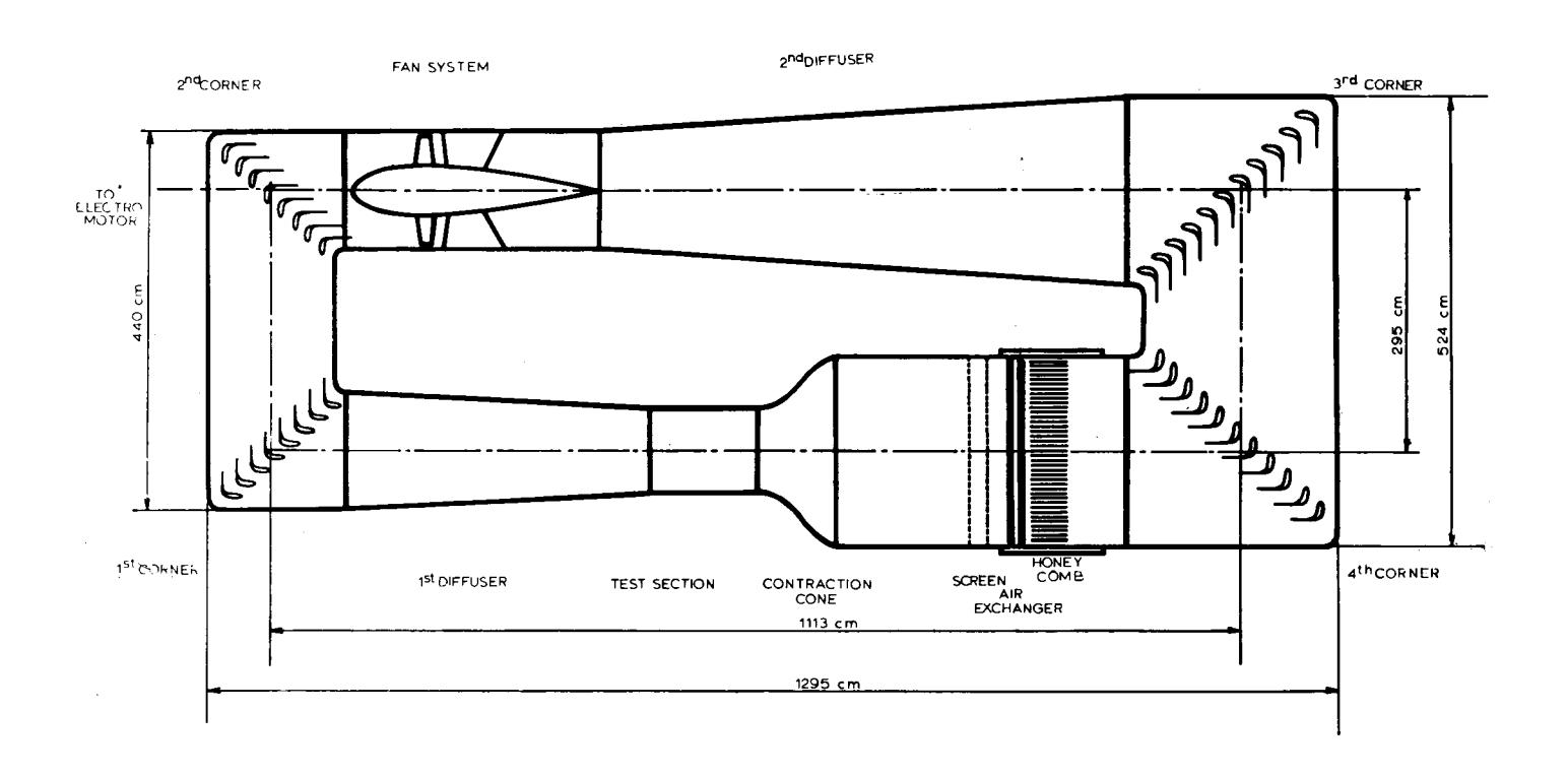
Figure 1. Schematic Diagram, Wind-Tunnel.
diffuser, the second corner, the third corner, the settling chamber with air-exchanger, honeycombs and screens, and the entrance cone. Each corner section is provided with turning vanes.
The cross section of most parts of the wind-tunnel is octagonal. The tunnel walls are built from steel plating strengthened by steel frames. The entire tunnel is placed indoor, and has a planview dimension of 12.95 m long by 5.24 m wide.
a. The Test-Section
The test-section has an octagonal cross section, with an average dimension of 1 m wide and 1 m high, or an equivalent diameter of 1.03 m. The length of the test-section is 1.30 m, and was made slightly tapered (the downstream equivalent diameter is 10 mm wider than the upstream equivalent diameter) to maintain constant pressure along the test-section. The test-section is provided with glass windows for viewing the model. The test-section is also equipped with a turntable to mount the model which can be adjusted manually. At present, due to the limitation imposed by the powerplant and the electric motor set up, a maximum velocity of 30 m/sec can be obtained at the test-section.
b. Power Losses
To calculate the power losses throughout the tunnel components, the method of Wattendorf (see ref. 1) was applied. The calculation was performed by R. Ramelan (2) to design the propeller fan and later verified by Marzwan Agus (3). The calculation procedure was to break down the tunnel into (1) cylindrical sections, (2) corners, (3) expanding sections and (4) contracting sections, and to calculate the loss for each.
The loss of energy in each section is usually written as a drop in static pressure, \(\Delta p\), or as coefficient of loss, K, which is the ratio between \(\Delta p\) and the dynamic head q. Wattendorf refers these local losses to the jet dynamic pressure, defining the coefficient of loss as:
\[K_{o} = \frac{\Delta p}{q} \cdot \frac{q}{q_{o}} = K \frac{q}{q_{o}}\]
Where subscript \(_{0}\) refers to the test-section, and K = \(\frac{\Delta p}{\frac{1}{2} \rho U^{2}}\). With the above definition, the energy loss at each section may be referred to the jet energy. As an indication of power losses in the tunnel, the energy ratio was defined as the ratio of the jet energy at the test-section to the summation of circuit losses. Following this procedure, power losses were computed for various velocities at the test-section.
For cylindrical section, the power loss can be expressed as:
\[K_o = \lambda \left(\frac{L}{D}\right) \left(\frac{A_o}{A}\right)^2\]
Where: L - the length of the section
D - the diameter or equivalent diameter
\(D_{\rm O}\) - the diameter of the test section
Ao - the area of the test-section
\(\lambda\) - coefficient of friction.
The friction coefficient can be evaluated following von Karman's formula:
\[\frac{1}{\sqrt{\lambda}} = 2 \log R\sqrt{\lambda} - 0.8\]
Since \(\lambda\) is dependent on Reynolds number, the latter should first be assumed. Note that this value of \(\lambda\) is valid for smooth cylindrical sections. Neglecting roughness effect, this formula was used for estimating power losses in the cylindrical sections including the test-section. For divergent sections, \(K_O\) is the summation of wall friction and expansion losses. Here:
\[K_0 = (\frac{\lambda}{8 \tan (\frac{\alpha}{2})} + 0.6 \tan \frac{\alpha}{2} (1 - \frac{D_1^4}{D_2^4}) \frac{D_0^4}{D_1^4}\]
Where: \(\alpha\) - the divergence angle between opposite walls
D<sub>1</sub> - smaller diameter
D<sub>2</sub> - larger diameter.
For corner sections with guide vanes:
\[K_0 = (0.10 + \frac{4.55}{(\log R)^{2.58}}) \frac{D_0^4}{D^4}\] which is partly empirical.
In the contraction cone the pressure drep is given by:
\[K_0 = 0.32 \lambda \frac{L_c}{D_0}\]
Where: \(\lambda\) - mean value of friction coefficient \(L_c\) - length of the contraction section \(D_0\) - diameter of the test-section.
Losses in the honeycomb are computed by using the following relationship:
\[K_{O} = K \frac{D_{O}^{4}}{D^{4}}\]
Where: \(D_{O}\) - diameter of the test-section
D - diameter of the settling chamber
K = 0.2 for honeycombs with hexagonal mesh and length to diameter ratio equal to 3.0.
Table 1 shows principal dimensions of various sections.
Table 1 Principal Dimensions of Various Sections
| Section | Diameter | Length | Divergence Angle | |
|---|---|---|---|---|
| Test-section | \(D_{o} = 1.03 \text{ m}\) | \(L_{\rm O} = 1.03 \text{ m}\) | ||
| First Diffuser | \(D_1 = 1.03 \text{ m}\) \(D_2 = 1.42 \text{ m}\) | L = 3.00 m | ||
| First Cylinder | D = 1.43 m | L = 1.10 m | ||
| Second Corner | D = 1.43 m | |||
| Second Cylinder | D = 1.43 m | L = 1.90 m | ||
| Second Diffuser | \(D_1 = 1.40 \text{ m}\) \(D_2 = 2.30 \text{ m}\) | L = 6.00 m | \[\tan \alpha = 0.075\] | |
| Third Corner | D = 2.30 m | |||
| Fourth Corner | D = 2.30 m | |||
| Settling Chamber | D = 2.30 m | L = 3.25 m | ||
| Contraction Cone | \(D_1 = 2.30 \text{ m}\) \(D_0 = 1.03 \text{ m}\) | L = 1.80 m | ||
Losses for various velocities are tabulated in table 2. This result can be employed to estimate the amount of power requi-red to drive the fan. It should be kept in mind that the above definition of the energy ratio excludes the losses occuri-ng at the fan nacelle and straightener system which should be taken into account in estimating the power required to drive the fan. The above definition of the energy ratio also excludes the efficiency of the electric motor driving the fan.
Table 2 Losses at wind-tunnel components for various velocities
| Test-section velocity (m/sec) | '15 | 18 | 20 | Z J | 26 |
| 1. Test-Section | 0.0147 0.0145 | 0"0143 0.0139 | 0.0136 | ||
| 2. First Diffuser | 0.0468 0.0464 | 0.04s9 0.04s1 | o.0444 | ||
| 3. First Corner | 0.0394 0.0391 | 0.0388 0.0386 | 0.0383 | ||
| 4. First Cylinder | 0.0002 0.0002 | 0.0002 0.0002 | 0.0002 | ||
| 5. Second Corner | 0.0394 0.0391 | 0.0388 0.0386 | 0.0383 | ||
| 6. Second Diffuser | 0.0159 0.0159 | 0.0158 0.0157 | 0.0r-56 | ||
| 7. Second Cylinder | 0.0004 0.0004 | 0.0004 0.0004 | 0.0004 | ||
| 8. Third Corner | 0.0425 0.0425 | 0.0424 0.0423 | 0.042L | ||
| 9. Fourth Corner | o.0425 0.0425 | 0.0424 0.0423 | o.042L | ||
| 10. Honeycombs | 0.0080 0.0080 | 0.0080 0.0080 | 0.0080 | ||
| 11. Screens | 0.0070 0.0070 | 0.0070 0.0070 | 0.0070 | ||
| 12. Fourth cylinder | 0.0006 0.0006 | 0.0006 0.0006 | 0.0006 | ||
| 13. Contraction Cone | 0.0065 0.0064 | 0.0063 0.0062 | 0.0060 | ||
| rKo | 0.2639 0.2626 | 0.2609 0.2589 | 0.2566 | ||
| 1/I K o | 3.79 | 3.80 | 3.83 | S.'80 | 3.90 |
| 307" Leakage | 1.14 | 1.14 | 1 .15 | 1.16 | L.T7 |
| Energy, Ratio | 2.65 | 2.66 | 2.68 | I 2.70 | 2.73 |
| Jet Energy, HP | 2,2 | 3.81- | 5.22 | 7 .95 | ir. st |
| Energy Loss, HI | 0.83 | 1.03 | 1 .95 | 2.95 | 4.23 |
| Measured Input Electric Motor HP | 3.38 | 5 .00 | 6 .8s | 9 .78 | L2.20 |
| Energy Loss/Input HP | o.246 0.206 0.285 0.302 | 0.347 |
c. Fan-Flow Straightener System
The fan is located downstream of the second corner, following the commonly accepted practice. This choice of the location of the fan was dictated by the following factors: 1) the fan develops its highest efficiency if it is located in a stream of fairly high velocity, 2) its cost is at least partially proportional to its diameter squared and 3) if the fan is to be driven by a motor outside the tunnel the corner location offers a short shaft length (1).
The fan of the present wind-tunnel is similar to a propeller of an airplane, and has four blades. Although the wind-tunnel fan seems similar to the propeller of an airplane, it operates under peculiar condition that place it in a class by itself, since the wind-tunnel fan is prevented by the law of continuity for incompressible fluid from producing an increase of velocity in the slip stream. The fan-flow straightener system employs a fan with straightener vanes behind it, without installation of prerotation vanes. For simplicity of construction, the fan blades as well as the straightener vanes are built as fixed pitched blades.
d. Fan Design
The fan diameter is \(1.40~\rm m\), and the fan section has an area of \(1.54~\rm m^2\). The fan boss diameter is \(0.84~\rm m\), which is similar to the diameter of the nacelle. The number of the fan blades is four, while there are seven straightener vanes. Table 3 shows the design calculation results. The design fan tip speed will be \(125~\rm m/sec\), which is well below the maximum allowable speed of \(500~\rm m/sec\), a figure suggested to avoid excessive compressibility effects.
e. The Straightener Vanes
It has been shown (1) that satisfactory anti-twist or straightener vanes can be made by using the NASA symmetrical airfoils set with their chords parallel to the tunnel centerline provided that the amount of twist to be removed is small compared to the axial velocity. The limiting twist is that required to stall the vanes, i.e. \(e=\omega r/u=\tan\tau\) (where \(\tau=\) angle of twist in the slip-stream and \(\omega=\) angular velocity in the slip-stream at radius r) must correspond to an angle less than \(\alpha\) of a symmetrical section at infinite aspect ratio including multiplane interference. The straightener vanes with constant thickness along the radius were designed, with thickness
ratio of 0.15. Table 3 also shows the dimension of the straightener vanes. The detail of the design was reported in references 2 and 3.
| tio of radial distance om the fan axis to the fan radius | 0.6 | 0.7 | 0.8 | 0.0 | 1.0 | ||
|---|---|---|---|---|---|---|---|
| Design Variables | , 0.7 | 0.0 | . 0.9 | 1.0 | |||
| \(\eta_{f}\) | - fan efficiency | 0.953 | 0.952 | 0.951 | 0.950 | 0.949 | |
| L/D | - lift to drag ratio | 44.8 | 52.5 | 54.5 | 60.2 | 63.5 | |
| Ø | - advance angle | 30°20' | 26°17' | 23°10' | 20°39' | 18°41' | |
| Cs | - chord of straightener vanes (m) **) | 0.382 | 0.446 | 0.506 | 0.573 | 0.636 | |
| ts | - thickness of straightener vanes (m) **) | 0.075 | 0.075 | 0.075 | 0.075 | 0.075 | |
| ω |
| 15.02 | 11.04 | 8.45 | 6.67 | 5.41 | |
| vT |
| 49.6 | 58.9 | 67.9 | 77.0 | 85.9 | |
| vR | - relative resultant velocity | 57.5 | 65.6 | 73.8 | 82.4 | 90.8 | |
| \(\alpha_{o}\) | - angle of attack | 1° | 2° | 2°48′ | 3°30' | 4° | |
| С |
| 0.195 | 0.158 | 0.125 | 0.103 | 0.093 | |
| β | - geometric helix angle of fan blade | 31°20' | 28°17' | 25°58' | 24°9.' | 22°4' | |
*) from ref. 2
**) from ref. 3
f. The nacelle
Following a recommendation in ref. 1, the nacelle diameter behind the fan was chosen to be 0.6 times the diameter of the fan, i.e. 0.84 m; the nacelle has a length of 1.40. The return passage where the nacelle is located has a diffusion angle of 7°.
g. Corner vanes, honeycombs and screens
The corner vanes were made from wood; the turning angle of the fourth corner vanes can be adjusted: The honeycombs were located upstream of the fourth corner vanes, with grid size of 14 cm equivalent diameter and 40 cm long. Two screens of gauze wire 36 grids per cm\(^2\) were installed downstream of the honeycomb.
III. SOME PERFORMANCE EVALUATION
3.1. Scope and Objectives
Having completed most parts of the design and construction, evaluation should be made on the extent to which design specification are met in order to obtain further information regarding future modifications and improvements. Since access to elaborate instrumentations is limited, the evaluation procedure involves the use of modest instrumentation, such as pitot tube and multiple manometer. The main objectives in performing the tests were:
- 1. to evaluate the uniformity of flow in the test-section.
- to evaluate the performance of the wind-tunnel, in particular to determine the relationship between power and velocity.
Some modifications were also performed to obtain a reasonable degree of flow uniformity.
3.2. Test Procedure and Instrumentation
The present investigation requires only the use of pitot tube, fluid multiple manometer (which was built at the mechanical engineering workshop) and thermometer. The control desk of the wind-tunnel allows adjustment of the voltage and current of the direct current motor. The automotive engine is controlled separately to vary the horse-power supplied to the electric motor. These adjustments were made to vary the wind-speed at the test-section.
During the course of the series of tests, some modifications were made. The turning vanes of the fourth corner were made adjustable, and were adjusted to obtain the desired degree of flow uniformity at the test-section. In addition two
screens were installed ln succession in the settlLng chamber of the honeycomb.
3.3. Results cnd Diseussion
I F
I'
Several readings were perfornred to investl-gate the velocity fluctuations at the test-sectj-on. Results from these tests indicate that the l"nstallation of Ehe screens has improved the average velocity variation of the flow at the test-sectlon from more than 2% (without the screen, wlth adjustnent of the turnlng vanes at the fourth corner), to less than 1%. A typica1 velocity distribution at the test-sectlon ls shollrt ln flgure 2, which was obtalned for electrlc motor horse-power of 14.5 HP and speed of 93b rpn; the correspo+ding average fl-olt velocity at the test-sectlon was 30 rn/sec. It was al-so observed, that the veloclty possesses an unsteadiness of 27",
Flgure 3 shows veloclty dlstributlon at a second station. The second statlon ls located at 20 cm downstream of the first sectlon, whlch ls l-ocated halfway along the test-section. At the second statlon, the average veloclty varlatlon has lncreased to 0.761, as compared to 0.5% at the flrst station. Veloclty dlstrlbutlon at these sectlons suggests the presence of some secondary flow.
Table 4 shows varlation of-statlc presdure along the test-sectlon. The indlcated decreabe of static pressure of less than 1% between extreme ends of the test-section can be considered satlsfactory. The amount of pressure drop al_ong
Table 4 Varlation of Statlc Pressure Along the Test-Section (ln lnches of water)
| Dlstance from (crn) lnlet section | n=900 nP=3.38 | n=l-000 HP=4.77 | n=1100 IIP=6 .31- | n=1200 HP=9.L2 | n=1300 HP=11.73 |
|---|---|---|---|---|---|
| 0 | 0.895 | 1 .005 | L.235 | 1 .615 | t.920 |
| 10 | 0.915 | 1.010 | I.245 | 1.610 | L,925 |
| 20 | 0 .915 | 1.010 | L,245 | 1 .615 | 1.945 |
| 30 | 0.915 | l015 | L.245 | t,620 | r965 |
| 40 | 0.915 | 1.015 | r,245 | 1.505 | 1.955 |
| 50 | 0.915 | L.025 | L.235 | 1.595 | 1.960 |
| 60 | 0.895 | 1.005 | 1,230 | L.57 5 | 1.950 |
| 70 | 0.895 | 1 .005 | L.225 | L.575 | 1.955 |
Figure 2. Velocity Contour at the Test Section measured at the center of the Test Section. Average velocity = 30.15 m/sec with standard deviation of = 0.45%.
Figure 3. Velocity Contour stream of the 30.13 m/sec with at the Test Sectlon, 20 cm downcenter Section. Average velocity standaril deviation of 0,70%.
the test-section bhoul-d be taken into consideratlon.for correctlng drag measurement. The three dlmenslonal. extent of the flow should be investlgated further by using a yaw probe.
The variation of electric motor horse-power to wlnd-speed at the test-section is shown in flgure 4, which also describes calculated estimation as tabulated in table 2. Discrepancy with calculated estimation ls considerable. This discrepancy should be subject to further work, but soue remarks are in order.
Part of this dlscrepancy may be due to inaccuraci-es in esti"mating the energy ratlo, which also lndlcates the discrepancies between estimated loss-factor and true l-oss-factor at wind-tunnel- components. Losses occuring at the corner sectlon wtth stationary turning vanes can be larger than estimated if the vanes r{ere improperly positloned during installation. Ilowever most of this dlscrepancy is believed to be due to unfavourable flow entering the fan (since the entrance nacelle upstream of the fan is not smooth), lower efficlency of the fan at off design condition and losses in the electric motor.
The performance of the present propeller fan shoul-d be evaluated before performing any rnodification to increase the capabillties of the fan. Originally lt raas designed to obtain a velocity of'40 m/sec in the test-section (2). However at present only a maxlmum velocity of 30 m/sec was obtained.
This situation is believed to be partly due to the limitations imposed by the combustion engine and the generator, and partly due to the off design fJ-ow situations upstream of the fan. The power plant set up was assembled by using second hand engine, generator and el-ectric motor. Although each of them has been repaired and reconditioned, their capabllities, are still lirnited. The comlustion engine ernployed in the present set up is a 1948 model of truck engine made by Chrys-1er corporation. The electric motor ls capable of delivering no more than 28 HP to the fan shaft. The propeller fan was designed by a staff member at the Mechanical Engineering Department (2) and manufactured local-J-y.
IV. CONCLUSIONS AND RECOMMENDATIONS
The following conclusions can be drawn:
1. The development of the low-speed wind-tunnel at ITB has reached a stage where a reasonably uniform velocity for educational purposes can nord be obtained at the test-section. The rnean velocity at the test-section was less than 12, while unsteadiness has been reduced to about 2%. The frequency of the unsteadiness was about 30 cycles per minute at test-section veloci-tv of 26 m/sec.
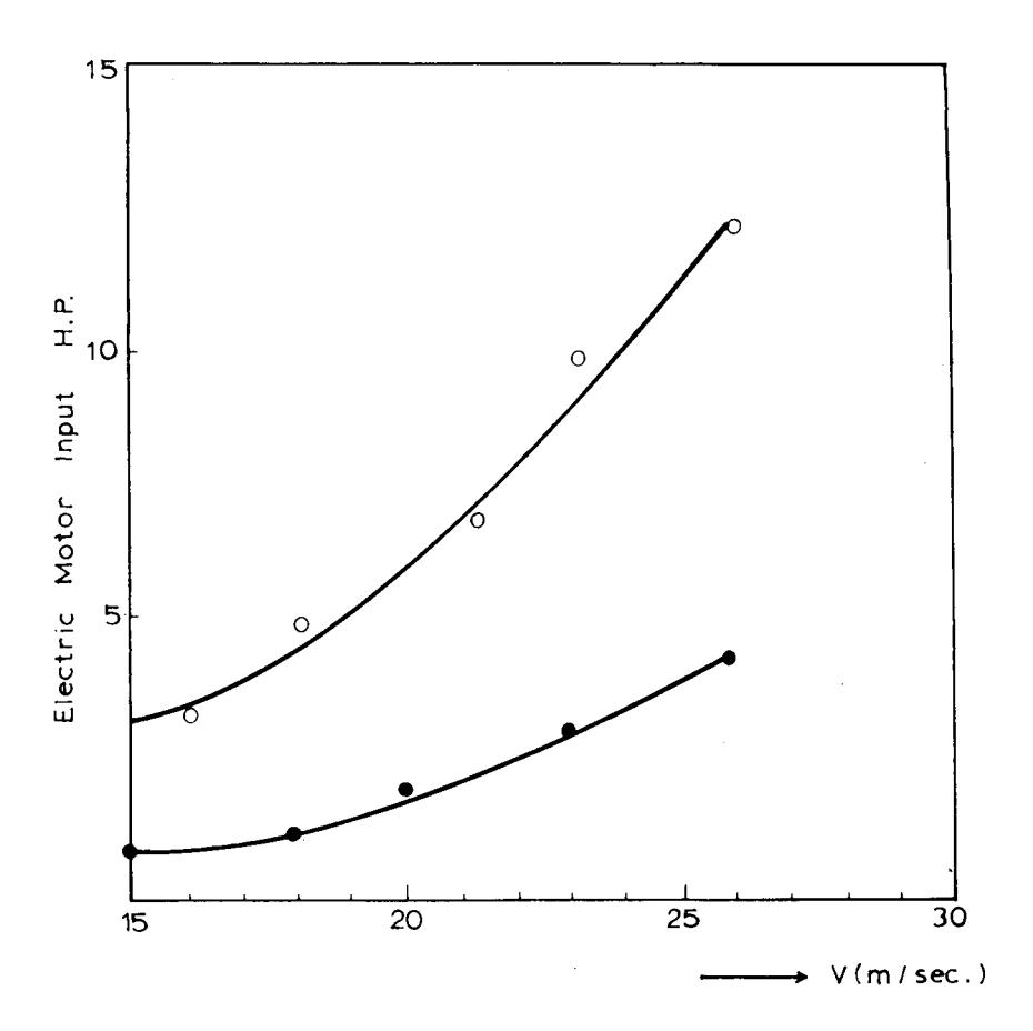
Figure 4. Power-Velocity relation
- t The maximr:m velocity obtained at the empty test-sectlon with the present power plant was 30 n/sec;
- 3 . The statlc pressure varlation along the tunnel was wlthln 2% of tt.e mean statlc pressure.
The following are reconmended for future work:
- 1 . Several tests shoul-d be made to evaluate the perfomance of the propeller fan and to perform some nodlficatlon.
- 2 . Further t.est should be conducted to evaluate and reduce secondary flow effects. Partlcular attention should be focussed on the flow along fan-straightener vanes systeu.
- 3 . Effort should be made to reduce flow unsteadiness at the test-sectlons, posslbly by lntroducing additlonal honeycombs at the expense of additlonal porder losses.
- 4 . Turbulence and boundary layer measurement should also be performed in the near future.
V. ACKNOWLEDGEMENT
The author would llke to acknowledge ir. 0. Dlran for providing useful infornatl,ons. Mr. Marzwan Agus has assisted the author'in performing some of the tests and urodiflcation of the wind-tunnel sections, while Mr. Roedlono K. Djatlkoesoemo has assisted the author in calibratl-ng the flow at the testsectlon.
VI. REFERENCES
- 1. Alan Pope: Itlow-Speed Wlnd-Tunnel Testlngtr, John WiJ-ey & Sons Inc., 1968.
- Roedianto Ramelan: trDeslgn of a Fan-Stralghtener System for the ITB Subsonic Wlnd-Tunnel", unpublished report, Mechanical Engineering Department, ITB, 1968.
- Marzwan Agus: "Evaluation of the Performance of the Wlnd-Tunne1", Mechani,cal Bngineer Thesis, Department of Mechanical Engineering IlB, L972 (in Indonesian). 3 .
(Receiued 22na June L973)