

I. INTRODUCTION
In an effort to develop satellite orbital computational program for satellite design studies, a computation scheme will be set up to calculate geostationary satellite orbits. The orbit of geostationary satellite will be influenced by earth's gravitational field, the gravitational field of the moon and the sun, and solar radiation pressure.
The earth's gravitational anomaly, the gravitational fields of moon and the sun, and solar radiation pressure will give rise to perturbation forces that perturb the orbit from its general elliptic shape. Specifically, the satellite orbit will not be truly geostationary, and the satellite will experience some drift.
In the present work, only the earth's gravitational anomaly will be taken into account, while perturbation due to the gravitational fields of the moon and the sun and solar radiation pressure will be dealt with in the future. The earth's gravitational potential will be represented as spherical harmonics (1) (2) (3).
*) Lecturer and Head, Aero & Hydrodynamics Laboratory, Institute of Technology Bandung,
**) Student, Department of Mechanical Lugineering, Institute of Technology Bandung.
The computational scheme outlined is a straight forward one. Several earth models will be utilized, and the accuracy of the computational program will be investigated.
II.GOVERNING EQUATIONS
Since the geostationary satellite considered is moving in the same direction as the direction of earth's rotation, it will be of great advantage to utilize a frame of reference rotating with the earth. It is then decided to use geocentric coordinate system which rotates with an angular speed \(\omega_e\) which has the same magnitude and direction as the earth's rotational speed, as shown in Figure 1.
Figure 1 Coordinate System
For origin located at the center of mass of the earth, the gravitational potential can be expressed by \(^{\{1\}\{2\}\{3\}}\).
\[V = -\frac{\mu}{r} \left[ 1 + \sum_{n=2}^{\infty} \sum_{m=0}^{n} \left( \frac{R}{r} \right)^{n} P_{nm} \left( \cos \theta \right) \right]\] \[\cdot \left( C_{nm} \cos m \lambda + S_{nm} \sin m \lambda \right)\] (1)
where:
r geocentric radius
? earth's equatorial radius
\(\theta\) collatitude
\(\mu\) product of the gravitational constant and the mass of the earth (=kM)
\(P_{nm}\) associated Legendre polynomials \(C_{nm}\), \(S_{nm}\) – satellite coefficients (tesseral harmonic coefficients)
and:
\[P_n(x) = \frac{1}{2^n n!} \frac{d^n}{dx^n} (x^2 - 1)^n; P_{nm}(x) = (1 - x^2)^{m/2} \frac{d^m P_n(x)}{dx^m}\]
Now letting:
\(J_n = -C_{no}\), the zonal harmonic coefficients
\[J_{nm} = (C_{nm}^2 + S_{nm}^2)^{1/2}\]
\[\lambda_{nm} = \frac{1}{m} \tan^{-1} (S_{nm}/C_{nm})\] the tesseral harmonic coefficients can be eliminated from equation (1) which is then recast into the following form:
\[V = -\frac{\mu}{r} \left[ 1 - \sum_{n=2}^{\infty} J_n \left( \frac{R}{r} \right)^n P_n \left( \cos \theta \right) + \sum_{n=2}^{\infty} \sum_{m=1}^{n} J_{nm} \left( \frac{R}{r} \right)^n P_{nm} \left( \cos \theta \right) \cos m (\lambda - \lambda_{nm}) \right]\] (2)
The kinetic energy per unit mass of satellite in an orbit around the earth can be represented by:
\[E_{k} = 1/2[\dot{r}^{2} + r^{2}\dot{\theta}^{2} + r^{2}\sin^{2}\theta(\dot{\lambda} + \omega_{e})^{2}]\] (3)
The corresponding total energy per unit mass can generally be represented by:
\[E = E_k - V \tag{4}\] where V is the potential energy per unit mass which is equivalent to the earth's gravitational potential at the satellite center of mass.
The equation of motion of the satellite can then be derived by utilizing Lagrange equation (4), i.e.:
\[\frac{d}{dt} \left( \frac{\partial E}{\partial r} \right) - \frac{\partial E}{\partial r} = 0\]
\[\frac{d}{dt} \left( \frac{\partial E}{\partial \dot{\lambda}} \right) - \frac{\partial E}{\partial \lambda} = 0\] \[\frac{d}{dt} \left( \frac{\partial E}{\partial \dot{\theta}} \right) - \frac{\partial E}{\partial \theta} = 0\] (5)
where r, \(\lambda\) dan \(\theta\) are spherical coordinates commonly utilized.
Substituting equation (3) in equation (4) and taking its derivatives in spherical coordinates and their time derivates, one obtains:
\[\frac{\partial E}{\partial r} = r \dot{\theta}^2 + r (\dot{\lambda} + \omega_e)^2 \sin^2 \theta - \frac{\partial V}{\partial r}\] \[\frac{\partial E}{\partial \dot{r}} = \dot{r}\] \[\frac{\partial E}{\partial \dot{\lambda}} = -\frac{\partial V}{\partial \lambda}\] \[\frac{\partial E}{\partial \dot{\lambda}} = r^2 (\dot{\lambda} + \omega_e) \sin^2 \theta\] \[\frac{\partial E}{\partial \theta} = r^2 (\dot{\lambda} + \omega_e)^2 \sin \theta \cos \theta - \frac{\partial V}{\partial \theta}\] \[\frac{\partial E}{\partial \dot{\theta}} = r^2 \dot{\theta}\] (6)
Substitution of equation (6) into equation (5) yields:
\[\ddot{r} - r \dot{\theta}^2 - r (\dot{\lambda} + \omega_e)^2 \sin^2 \theta + \frac{\partial v}{\partial r} = 0\] (7)
\[\frac{d}{dt} \left[ r^2 \left( \dot{\lambda} + \omega_e \right) \sin^2 \theta \right] + \frac{\partial v}{\partial \lambda} = 0\] (8)
\[\frac{d}{dt} (r^2 \dot{\theta}) - r^2 (\dot{\lambda} + \omega_e)^2 \sin \theta \cos \theta + \frac{\partial v}{\partial \theta} = 0\] (9)
To obtain a general solution, it is convenient to recast equations (7) to (9) into nondimensional forms by defining the following dimensionless parameters:
\[Z = \frac{r}{R}\] \[\tau = \omega_{c} t \tag{10}\]
\[\alpha = \frac{\mu}{\omega_a^2 R^3}\]
We then obtain:
\[z - z \theta^{2} - (1 + \lambda)^{2} z \sin^{2} \theta + \frac{\alpha}{z^{2}} \left[1 - \sum_{n} \frac{(n+1)J_{n}}{z^{n}} P_{n} (\cos \theta) + \sum_{n} \sum_{m} \frac{(n+1)J_{nm}}{z^{n}} P_{nm} (\cos \theta) \cos m (\lambda - \lambda_{nm})\right] = 0\] \[\frac{d}{d\tau} \left[(1 + \lambda) z^{2} \sin^{2} \theta\right] + \alpha \sum_{n} \sum_{m} \frac{m J_{nm}}{z^{n+1}} P_{nm} (\cos \theta)\] \[\cdot \sin m (\lambda - \lambda_{nm}) = 0\] \[(12)\]
\[\frac{d}{d\tau} (z^2 \dot{\theta}) - (1 - \dot{\lambda})^2 z^2 \sin \theta \cos \theta - \alpha \sum_{n} \frac{J_n}{z^{n+1}} \sin \theta P'_n (\cos \theta)\] \[+ \alpha \sum_{n} \sum_{m} \frac{J_{nm}}{z^{n+1}} \sin \theta P'_{nm} (\cos \theta) \cos m (\lambda - \lambda_{nm}) = 0\] (13)
where the dotted variables indicate their derivatives with respect to dimensionless time \(\tau\). These are the governing equations of motion of the satellite.
III. RADIUS OF SYNCHRONOUS ORBIT
The radius of synchronous orbit is the distance between the satellite and center of mass of the earth at which the radial acceleration due to kinetic (angular motion) and potential (gravitational potential) energy is zero. Since in addition a true geosynchronous orbit lies in the equatorial plane (\(\theta = 90^{\circ}\)), then equation (11) reduced to:
\[z - (\frac{\alpha}{z^2}) \left[1 - \sum_{\substack{n \text{even}}} \frac{(n+1) J_n A_n}{z^n}\right]\]
\[+\sum_{\substack{n-m \\ \text{even}}} \frac{(n+1)J_{nm} A_{nm}}{z^n} \cos m (\lambda - \lambda_{nm}) = 0\] (14)
where even subscript signifies even values; in equation (14), we have taken advantage of the fact that for \(\theta = 90^{\circ}\),
\[P_{n}(\cos \theta) = A_{n} = \frac{(-1)^{n/2} n!}{2^{n} (\frac{n}{2})! (\frac{n}{2})!}\] for n even \[P_{nm}(\cos \theta) = A_{nm} = \frac{(-1)^{(n-m)/2} (n+m)!}{2^{n} (\frac{n-m}{2})! (\frac{n+m}{2})!}\] for \((n-m)\) even (15) \[P_{n}(\cos \theta) = P_{nm}(\cos \theta) = 0\] for \(n\) and \((n-m)\) odd
Equation (14) can be solved by numerical approach to give the values of the radius of synchronous orbits Z for any value of longitude \(\lambda\).
Longitudinal Acceleration
At any longitudinal position, the longitudinal acceleration of the satellite can be calculated from equation (12), which can be rewritten into:
\[\ddot{\lambda} = -\frac{\alpha}{z^2 \sin^2 \theta} \sum_{n=m}^{\infty} \frac{m J_{nm}}{z^{n+1}} P_{nm} (\cos \theta) \sin m (\lambda - \lambda_{nm})\] (16)
or, noting that \(\theta = 90^{\circ}\):
\[\ddot{\lambda} = -\alpha \sum_{\substack{n-m \text{even}}} \frac{m J_{nm} A_{nm}}{z^{n+3}} \sin m (\lambda - \lambda_{nm})\] (17)
Using the value of Z obtained from equation (14), them equation (17) can be readily evaluated.
IV. STATIONARY CONDITIONS
Equation (11), (12) and (13) contain stationary conditions, at which the satellite experiences no radial acceleration, and its angular velocity exactly equals to the angular velocity of the earth. Such condition is represented by sets of values of Z, \(\theta\) and \(\lambda\) which are constant, i.e.:
\[z = z_0 = \text{constant}\]
\(\lambda = \lambda_0 = \text{constant}\) (18)
\(\theta = \theta_0 = \frac{\pi}{2} - \delta_0 = \text{constant}\)
where \(\delta\) is the geocentric lattitude, which is not zero, although small. In the geocentric frame of reference which rotates with the earth, then \(\ddot{Z}\), \(\dot{Z}\), \(\dot{\lambda}\), \(\dot{\lambda}\), \(\dot{\theta}\) and \(\dot{\theta}\) are equal zero, thus reducing equations (11), (12) and (13) to:
\[z_{0} \cos^{2} \delta_{0} - \frac{\alpha}{z_{0}^{2}} \left[1 - \sum_{n} \frac{(n+1)J_{n}}{z_{0}^{n}} P_{n} (\sin \delta_{0}) + \sum_{n} \sum_{m} \frac{(n+1)}{z_{0}^{n}} \right]\] \[. J_{nm} P_{nm} (\sin \delta_{0}) \cos m (\lambda_{0} - \lambda_{nm}) = 0\] (19)
\[\sum_{n=m}^{\infty} \frac{m J_{nm}}{z_0^n} P_{nm} (\sin \delta_0) \sin m (\lambda_0 - \lambda_{nm}) = 0\] (20)
\[z_0^2 \sin \delta_0 + \alpha \sum_n \frac{J_n}{z_0^{n+1}} P'_n (\sin \delta_0) - \alpha \sum_n \sum_m \frac{J_{nm}}{z_0^{n+1}} P'_{nm} (\sin \delta_0)\] \[\cdot \cos m (\lambda_0 - \lambda_{nm}) = 0\] (21)
Since the shape of the earth is almost symmetrical and the value of \(J_{nm}\) is small, then \(\delta_0\) can be expected to be small. Hence the values of the Legendre and its associated polynomials in \(\delta_0\) can be approximated, following Blitzer \(^{(5)}\), by:
(22)
\[\begin{split} P_n & (\sin \delta_0) = A_n \\ P_{nm} & (\sin \delta_0) = A_{nm} \\ P'_n & (\sin \delta_0) = D_n \delta_0 \\ P'_{nm} & (\sin \delta_0) = D_{nm} \delta_0 \\ P_n & (\sin \delta_0) = B_n \delta_0 \\ P_{nm} & (\sin \delta_0) = B_{nm} \delta_0 \\ P'_n & (\sin \delta_0) = B_n \delta_0 \\ P'_n & (\sin \delta_0) = B_n \\ P'_{nm} & (\sin \delta_0) = B_n \end{split}\] for n and (n - m) odd where:
\[A_{nm} = \frac{(-1)^{n/2} n!}{2^{n} (\frac{n}{2})! (\frac{n}{2})!}\] \[A_{nm} = \frac{(-1)^{(n-m)/2} (n+m)!}{2^{n} (\frac{n-m}{2})! (\frac{n+m}{2})!}\] \[B_{n} = \frac{(-1)^{(n-1)/2} (n+1)!}{2^{n} (\frac{n-1}{2})! (\frac{n+1}{2})!}\] \[B_{nm} = \frac{(-1)^{(n-m-1)/2} (n+m+1)!}{2^{n} (\frac{n-m-1}{2})! (\frac{n+m+1}{2})!}\] \[D_{n} = \frac{(-1)^{(n+2)/2} (n+2)! (n^{2}+n)}{2^{n+1} (\frac{n}{2})! (\frac{n+2}{2})! (n+1)}\] \[D_{nm} = \frac{(-1)^{(n-m+2)/2} (n+m+2)! (n^{2}-m^{2}+n)}{2^{n+1} (\frac{n-m}{2})! (\frac{n+m+2}{2})! (n+m+1)}\]
Substituting these values in equations (19) to (21), one obtains:
\[z_{0}^{3} - \alpha \left[1 - \sum_{\substack{n \text{even}}} \frac{(n+1) J_{n} A_{n}}{z_{0}^{n}} + \sum_{\substack{n \text{even}}} \frac{(n+1) J_{nm} A_{nm}}{z_{0}^{n}} \cos m \left(\lambda_{0} - \lambda_{nm}\right)\right] = 0\] (24)
\[\text{[rumus tidak dapat ditampilkan dengan baik — lihat PDF asli]}\] (25)
\[z_0^3 \delta_0 + \alpha \sum_{\substack{n \ \text{odd}}} \frac{J_n B_n}{z_0^n} - \alpha \sum_{\substack{n \ \text{odd}}} \frac{J_{nm} B_{nm}}{z_0^n} \cos m (\lambda_0 - \lambda_{nm}) = 0\] (26)
Equations (24), (25) and (26) can be solved numerically to obtain the sets of stationary values \((z_0, \lambda_0, \delta_0)\).
V.MOTION AROUND STATIONARY POINTS
In reality, the motion of geostationary satellite is not truely geostationary, but drifting around its geostationary positions. Such a condition can be represented by:
\[z = z_0 + \Delta\] \[\lambda = \lambda_0 + \phi\] \[\delta = \delta_0 + \beta\] (27)
where \(\Delta \ll 1\), \(\phi \ll \pi\) and \(\beta \ll \pi\)
To obtain this motion, equation (26) is substituted into equations (24) (25)
and (26) and then linearizing by ignoring square and product terms in \(\triangle\), \(\phi\), \(\beta\), and their derivatives, we find (5):
\[\ddot{\Delta} - (1 + a) \Delta - 2 z_0 \dot{\phi} + c \phi + e \beta = 0\] (28)
\[z_0^2 \ddot{\phi} + b \phi + 2 z_0 \ddot{\Delta} + c \Delta + f \beta = 0\] (29)
\[\ddot{\beta} + (1+k)\beta + (e/z_0^2)\Delta + (f/z_0^2)\phi = 0\] (30)
where:
\[a = \frac{2 \alpha}{z_0^3} \left[ 1 - \sum_{\substack{n \text{even}}} \frac{(n+1)(n+2) J_n A_n}{2 z_0^n} - \sum_{\substack{n \text{even}}} \frac{(n+1)(n+2) J_{nm} A_{nm}}{2 z_0^n} \cos m (\lambda_0 - \lambda_{nm}) \right]\]
\[b = \alpha \sum_{\substack{n-m \\ \text{even}}} \frac{m^2 J_{nm} A_{nm}}{z_0^{n+1}} \cos m (\lambda_0 - \lambda_{nm})\]
\[c = -\alpha \sum_{\substack{n-m \\ \text{even}}} \frac{m(n+1)J_{nm}A_{nm}}{z_0^{n+2}} \sin m(\lambda_0 - \lambda_{nm})\] (31)
\[e = -\alpha \sum_{\substack{n \text{odd}}} \frac{(n+1)J_nB_n}{z_0^{n+2}} + \alpha \sum_{\substack{n-m \text{odd}}} \frac{(n+1)J_{nm}B_{nm}}{z_0^{n+2}}\] \[\cdot \cos m (\lambda_0 - \lambda_{nm})\]
\[f = \alpha \sum_{n=1 \ n} \frac{m J_{nm} B_{nm}}{z_0^{n+1}} \sin m (\lambda_0 - \lambda_{nm})\]
\[k = \alpha \sum_{\substack{n \text{even}}} \frac{J_n D_n}{z_0^{n+3}} - \alpha \sum_{\substack{n-m \text{even}}} \frac{J_{nn_1} D_{nm}}{z_0^{n+3}} \cos m (\lambda_0 - \lambda_{nm})\]
Equations (28) to (30) can be solved if the initial conditions \(\Delta_0\), \(\dot{\Delta}_0\), \(\phi_0\), \(\dot{\phi}_0\), \(\beta_0\) and \(\dot{\beta}_0\), are known, and hence the position, velocity and acceleration of the satellite during the course of its motion can be determined.
VI. DATA AND COMPUTATIONAL ASPECTS
Computational Scheme
Equation (14) can be solved for the radius of synchronous orbit Z by utilizing Regula Falsi method. Thus the values of Z for various longitudinal positions can be obtained and plotted. By substituting values of Z for any longitudinal positions in equation (16), one can obtain the longitudinal accelerations \(\lambda\).
The positions of stationary points \((z_0, \lambda_0, \delta_0)\) can be obtained from equations (25) and (26) for \(\lambda_0\) and \(\delta_0\), respectively. To obtain \(z_0\) values, an alternative method which is more expeditious than solving equation (24), and hence avoiding simultaneous solution of equations (24), (25) and (26) is utilized. For this purpose, \(z_0\) values are solved by identifying longitudinal positions where the longitudinal acceleration vanishes and employ these values to obtain \(z_0\).
Next, simultaneous differential equations (28), (29) and (30) which represent the equations of motion of the satellite about its stationary points, are solved by utilizing Runge-Kutta method. For other points along the geosynchronous orbit the system of equations (11), (12) and (13) have to be solved instead of (28), (29) and (30) by using solutions of the latter system of equations as initial approximation. Direct solution of equations (11), (12) and (13) is presently being worked out.
Figure 2, 3 and 4 outline the algorithms used for the computational procedures mentioned above.
Earth and satellite coefficients data
Two sets of data are utilized in the computation; these are the earth and satellite coefficients data given by International Astronomical Union (IAU) in 1968, as tabulated in reference 6, reproduced in Table 1, and Goddard Earth Model 8 (GEM 8) published in reference 7, and reproduced in Table 2.
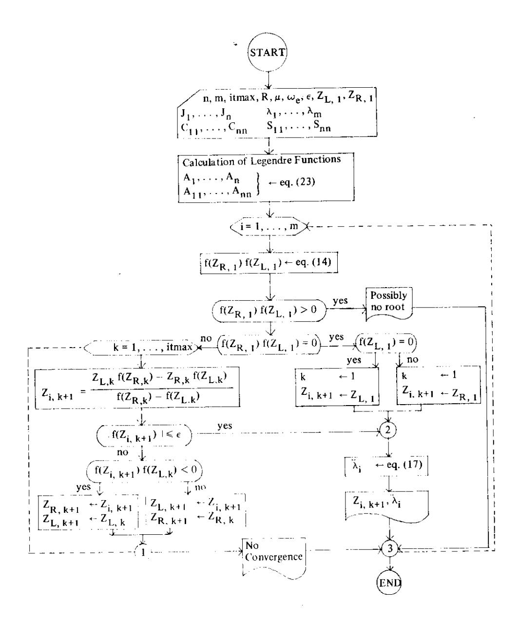
Figure 2 Flow chart for the solution of equation (14) with Regula-Falsi method.
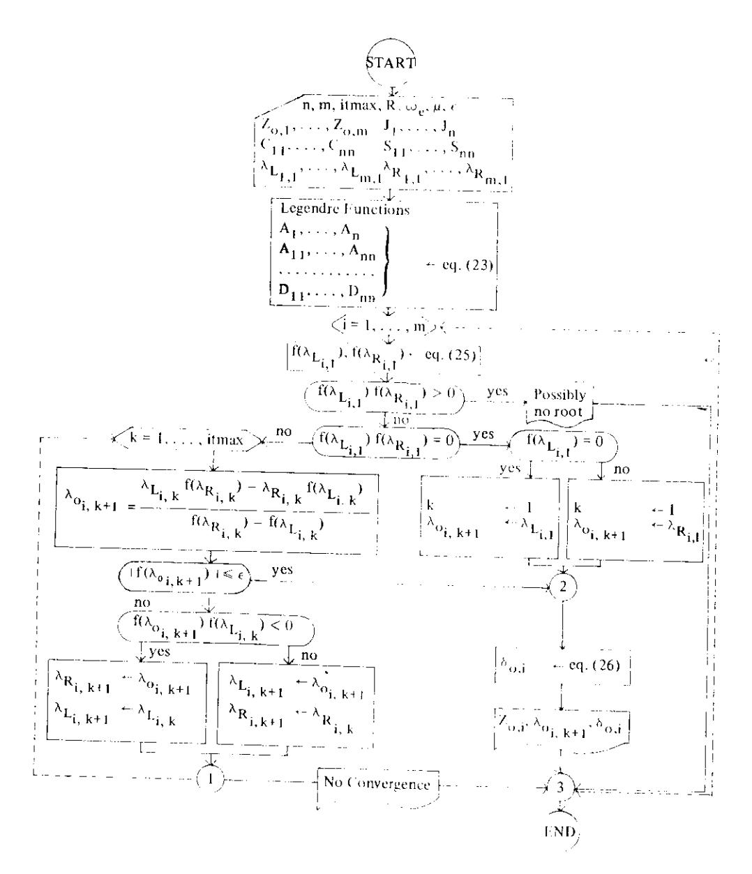
Figure 3 Flow chart for the solution of equation (25) using Regula-Falsi method
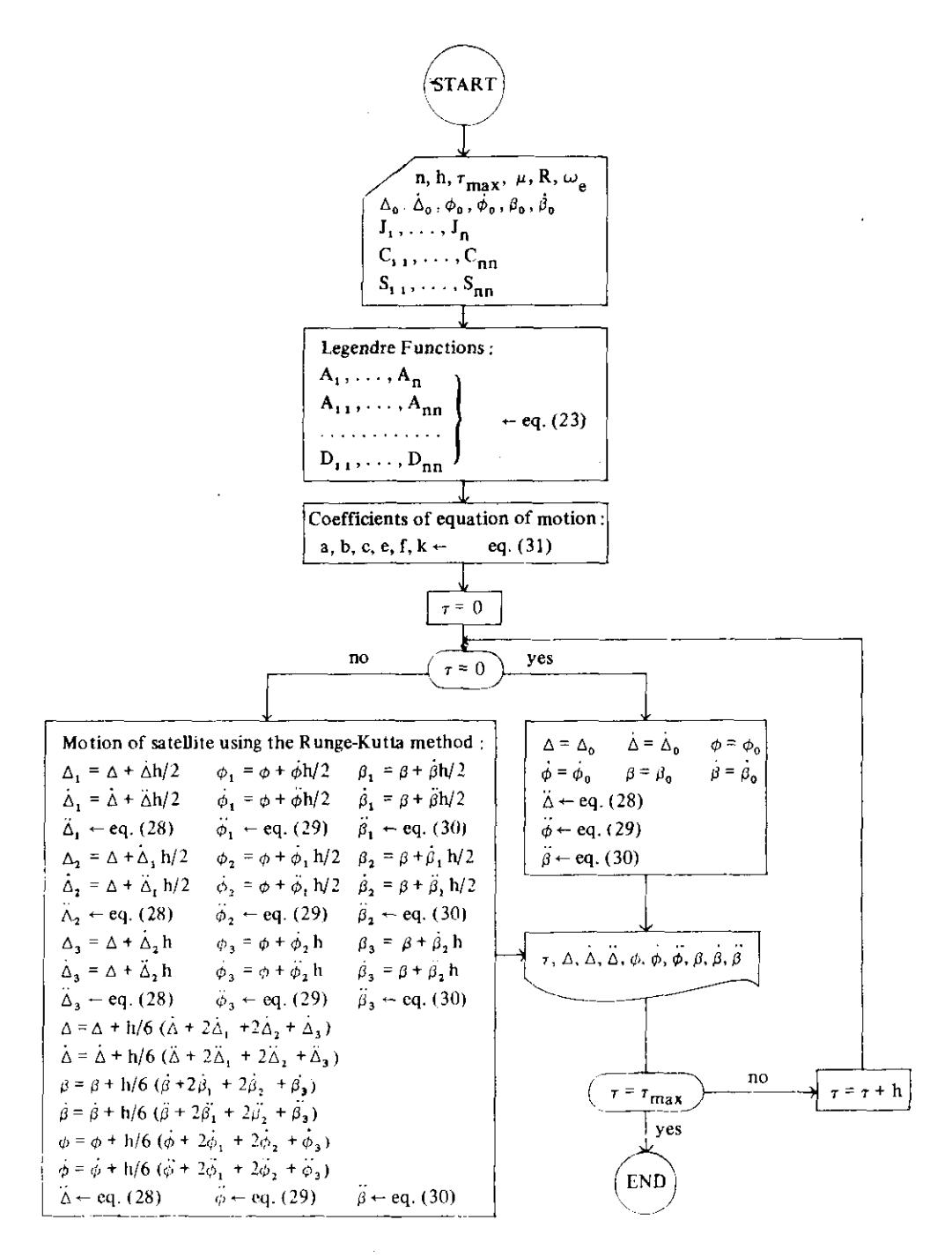
Figure 4 Flow chart for the solution of equation (28), (29) and (30) by using Runge-Kutta method
TABLE 1, Coefficients of the Geopotential for IAU 1968
| \(\mu =\) | 3.986 X | 105 | km3/sec2 | ²;R | = 6378 km |
|---|
| n | 106 Jn | nm | 106 Cnm | 106 Snm |
|---|---|---|---|---|
| 2 | 1082,70 | 21 | 0.0000 | 0,000,0 |
| 3 | - 2.56 | 22 | 1.5700 | - 0.8970 |
| 4 | ~ 1.58 | 31 | 2,1000 | 0.1600 |
| 5 | ~ 0,15 | 32 | 0.2500 | ~ 0.2700 |
| 6 | 0.59 | 33 | 0.0770 | 0,1730 |
| 7 | - 0.44 | 41 | - 0.5800 | - 0.4600 |
| 42 | 0.0740 | 0,1600 | ||
| 43 | 0.0530 | 0.0040 | ||
| 44 | - 0.0065 | 0.0023 | ||
TABLE 2. Coefficients of the Geopotential for GEM-8*
\(\mu = 3.986008 \times 10^5 \text{ km}^3/\text{sec}^2\); R = 6.378.145 km
| n | 106 Jn | n | m | 106 Cnm | 106 Snm |
|---|---|---|---|---|---|
| 2 | 1082,6254 | 2 | 1 | - 0.0001 | 0.0004 |
| 3 | - 2,5357 | 2 | 2 | 1.5710 | - 0,9007 |
| 4 | - 1,6200 | 3 | 1 | 2.1940 | 0,2696 |
| 5 | - 0.2259 | 3 | 2 | 0.3066 | - 0.2129 |
| 6 | 0.5426 | 3 | 3 | 0.0999 | 0.1976 |
| 7 | - 0.3613 | 4 | 1 | - 0.5098 | - 0.4495 |
| 8 | ~ 0,2066 | 4 | 2 | 0.0777 | 0.1489 |
| 9 | - 0.1142 | 4 | 3 | 0.0589 | - 0,0118 |
| 10 | - 0.2475 | 4 | 4 | - 0.0041 | 0.0065 |
| 29 | - 0.0238 | 30 | 28 | - 0.8558× 10-40 | \(0.1019 \times 10^{-4}\) |
Coefficients of the geopotential are derived from the normalized values given by GEM--8 (1977).
VII. DISCUSSION OF RESULTS
Taking into account the earth's gravitational anomaly, the radius of synchronous orbit r = ZR is obtained by solving equation (16) and shown in Figure 5. The values of r varies from 42164, 7830 km to 42164.7952 km, where the smallest value occurs at \(\lambda = 75^{\circ}\) and the largest value occurs at \(\lambda = 162.5^{\circ}\).
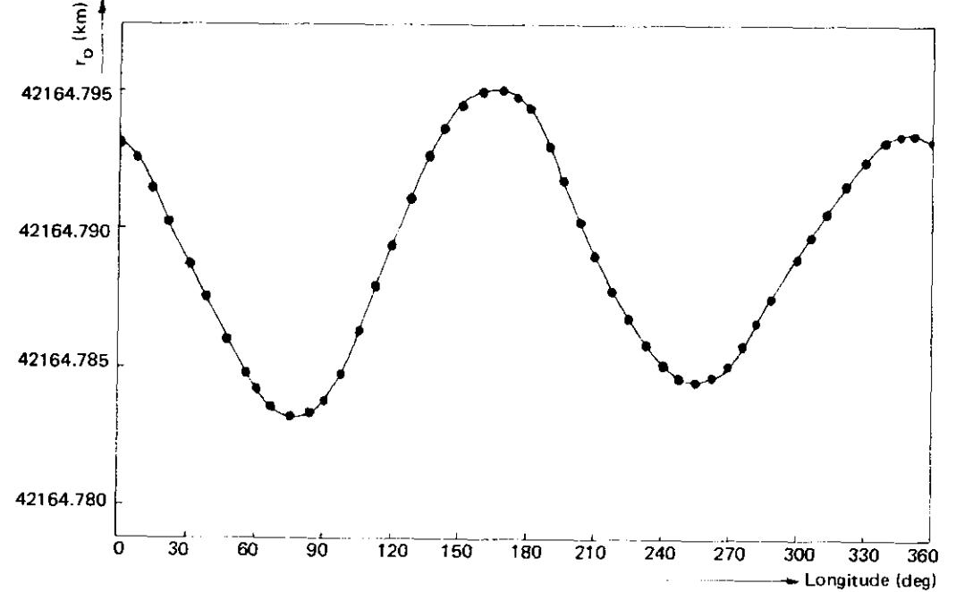
Figure 5 Radius of Synchronous Orbit
If the influence of the earth oblateness \((J_2)\) alone is taken into account, the radius of geosynchronous orbit turns out to be 42164.78687 km for any longitude. This value can be compared with the radius of Keplerian orbit (without considering the gravitational anomaly) of 42164.26687 km. Thus the influence of \(J_2\) is increasing the geosynchronous orbit by 520 m, while higher order terms of the gravitational anomaly increase the radius further by 516.13 m up to 528.33 m. It can be confirmed, that indeed the dominant value is due to \(J_2\).
Computational results for longitudinal acceleration \(\ddot{\lambda}\) as function of \(\lambda\) are shown in Figure 6. Here it can also be observed, that the largest contribution is due to \(J_{22}\). The values of longitudinal acceleration vary between \(-0.59007 \times 10^{-3} \, \text{degrees/day}^2\) and \(0.65853 \times 10^{-3} \, \text{degrees/day}^2\). For \(\lambda = 77.5^\circ\) up to \(160^\circ\) and for \(\lambda = 255^\circ\) up to \(347.5^\circ\), the satellite experiences an acceleration at the same direction as the rotational speed of the earth, while otherwise it experiences an acceleration in the opposite direction.
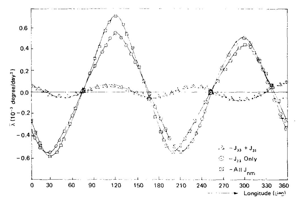
Figure 6 Longitudinal Acceleration
For Keplerian orbit, all points are stationary and located at the equatorial plane on a ring with a radius of \(r_0 = 42164.26687\) km. However, the influence of the gravitational anomaly reduces the number of stationary points to four, and they are not precisely located at the equatorial plane. Computational results for stationary points are tabulated in Table 3.
| TARL | E | 2 | Equilibrium | Positions | /CEM | Q١ |
|---|---|---|---|---|---|---|
| IADL | . = | Э. | - commorning | POSITIONS | I Call IV | A1 |
| Position | r0 ( km ) | λ0 (deg) | δ0 ( rad ) |
|---|---|---|---|
| 1 | 42164.7830 | 75.0238 | ~3.5880 × 10⁻⁸ |
| 2 | 42164.7952 | 162.0093 | 0.4805 × 10⁻⁸ |
| 3 | 42164.7847 | 254.7888 | -2.7790 × 10⁻⁸ |
| 4 | 42164.7936 | 348.3743 | 0.6912 × 10⁻⁸ |
The trajectories of the satellite about stationary points for various values of inclinalion i are shown in Figures 7:8 and 9.
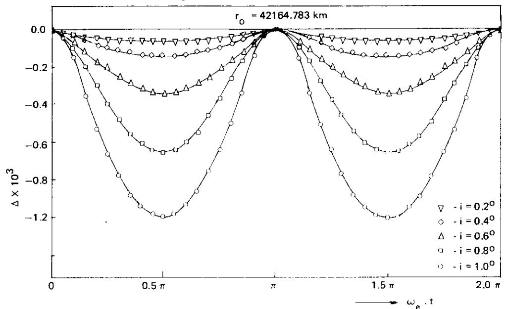
Variation of orbital radius as function of time Figure 7
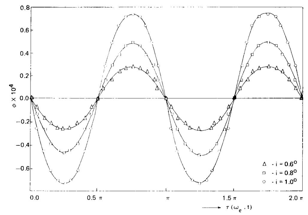
Figure 8 Longitude variation of stationary point as function of time
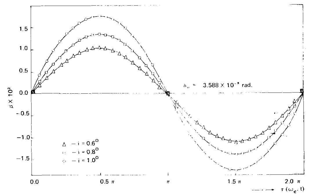
Figure 9 Variation of the lattitude of stationary point as function of time
These figures exhibit changes of satellite positions from its stationary points in one cycle (one revolution around the earth), which has a period of one day. The corresponding subsatellite trajectories (or ground tracks) with well known figure 8 configuration for various values of inclination i are shown in Figure 10; for larger inclination, the ground track is also larger.
Assessment of Computational Results
To assess the accuracy and validity of the computational scheme, comparison will be made with results obtained by previous workers. By employing data used by Blitzer \(^{(5)}\), i.e. \(J_n\) following King – Hele (1964) and \(J_{nm}\) following Izsak (1964) \(^{(5)}\), present results will be compared with Blitzer's \(^{(5)}\). Blitzer utilizes the following formula:
\[\lambda_{0} = \lambda_{22} + \frac{s \pi}{2} - \frac{\sum_{\substack{n=-m \text{even}}} \sum_{\substack{n=-m \text{even}}} \frac{m J_{nm} A_{nm}}{z_{0}^{n}} \sin m (\lambda_{22} - \lambda_{nm} + \frac{s \pi}{2})}{\sum_{\substack{n=-m \text{even}}} \sum_{\substack{n=-m \text{even}}} \frac{m^{2} J_{nm} A_{nm}}{z_{0}^{n}} \sin m (\lambda_{22} - \lambda_{nm} + \frac{s \pi}{2})}\] (32)
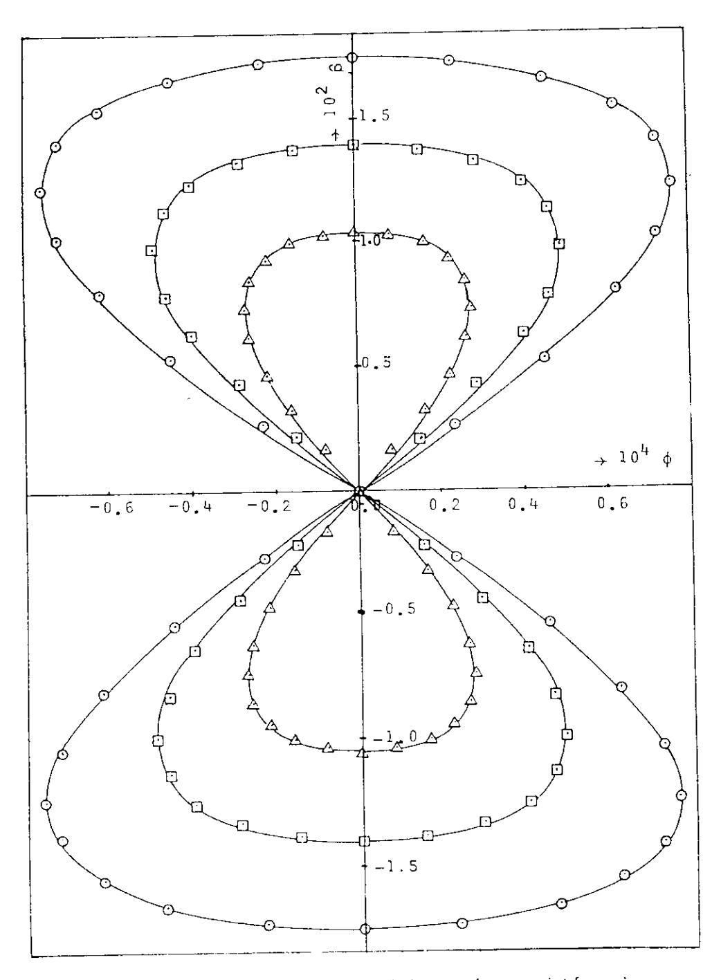
Figure 10 Ground track (subsatellite trajectory) about stationary point for various inclination of orbit.
\[\delta_0 = -\sum_{\substack{n \text{odd}}} \frac{J_n B_n}{z_0^n} + \sum_{\substack{n \text{odd}}} \sum_{\substack{n \text{odd}}} \frac{J_{nm} B_{nm}}{z_0^n} \cos m (\lambda_0 - \lambda_{nm})\] where s = 1, 2, 3, 4.
Using formula (32), Blitzer arrived at values of stationary positions shown in Table 4. If these values are substituted in equation (25), the right hand side will be equal to \(\simeq 10^{-9}\), while using similar basic data, we obtain values of stationary positions which are very close to Blitzer's results, as also shown in Table 4. However, if our values are substituted in equation (25), the right hand side will be closer to zero, i.e. \(10^{-18}\).
| TABLE 4. | Comparison o | f Equilibrium Position | results with Blitzer's |
|---|
| Present N | lethod | L. Blitzer's | ||||
|---|---|---|---|---|---|---|
| Position | Z0 | λο (deg) | \[10^4 \times \delta_0\] ( sec ) | λ0 (deg) | \[10^4 \times \delta_0\] ( sec ) | |
| 1 | 6.63 | - 15,201 | -10,456 | - 15,2 | -11 | |
| 2 | 6.63 | 75,052 | - 37,374 | 75,1 | - 37 | |
| 3 | 6,63 | 161,708 | - 15,823 | 161,7 | - 16 | |
| 4 | 6.63 | -110,861 | -43,965 | -110,9 | - 44 | |
The subsatellite trajectory results will be compared to Flury's. According to Flury \(^{(8)}\), the subsatellite trajectory is represented by
\[\delta r = \delta a - \delta ae \cos M = \delta a - \delta a \eta \cos \lambda - \delta a \xi \sin \lambda\]
\[\delta L = 2 e \sin M + (n - \omega_e) t = 2 \eta \sin \lambda - 2 \xi \cos \lambda + (n - \omega_e) t\]
\[\delta \phi = i \sin (\omega + M) = \beta \sin \lambda - \alpha \cos \lambda\] where:
\[\eta = e \cos (\Omega + \omega), \xi = e \sin (\Omega + \omega)\]
\[\alpha = \sin i \sin \Omega\], \(\beta = \sin i \cos \Omega\)
M = n t, n = mean motion
L = longitude
\(\lambda = (\Omega + \omega + M)\)
As indicated by Table 5, the agreement of our results with Flury's is indeed excllent.
TABLE 5. Comparison of Ground-Track results (GEM 8) with Flury's
| inclination (deg) | Present | Method | Flury's | ||
|---|---|---|---|---|---|
| width (rad) | height (rad) | width (rad) | height (rad) | ||
| 0,1 | 0,761545×10⁻⁶ | 0,349060×10⁻² | 0,761543×10⁻⁶ | 0,349065×10⁻² | |
| 0,2 | 0,304620×10⁻⁵ | 0,698100×10⁻² | 0,304617×10⁻⁵ | 0,698131×10⁻² | |
| 0,3 | 0,685388×10⁻⁵ | 0,104716×10⁻¹ | 0,685389×10⁻⁵ | 0,104719×10⁻¹ | |
| 0,4 | 0,121850×10⁻⁴ | 0,139620×10⁻¹ | 0,121860×10⁻⁴ | 0,139626×10⁻¹ | |
| 0,5 | 0,190385×10⁻⁴ | 0,174524×10⁻¹ | 0,190385×10⁻⁴ | 0,174532×10⁻¹ | |
| 0,6 | 0,274153×10⁻⁴ | 0,209420×10⁻¹ | 0,274155×10⁻⁴ | 0,209439×10⁻¹ | |
| 0,7 | 0,373153×10⁻⁴ | 0,244340×10⁻¹ | 0,373156×10 -4 | 0,244346×10⁻¹ | |
| 8,0 | 0,487380×10⁻⁴ | 0,279240×10⁻¹ | 0,487387×10⁻⁴ | 0,279252×10⁻¹ | |
| 0,9 | 0,616838×10⁻⁴ | 0,314140×10⁻¹ | 0,616850×10⁻⁴ | 0,314159×10⁻¹ | |
| 1,0 | 0,761525×10⁻⁴ | 0,349040×10⁻¹ | 0,761543×10⁻⁴ | 0,349065×10⁻¹ | |
Comparison of IAU 1968 and GEM 8 results
Satellite coefficients have now been obtained with increasing accuracy; the latest information known to the authors is known as GEM-10, with higher order coefficients in the range of hundredth. However, in the time of writing, only data of GEM-8 and IAU 1968 are available. Preliminary work using IAU 1968 data was reported in reference 9. Comparison of results using these sets of data and present method is intended to investigate further whether the computational accuracy is adequate.
Results are tabulated in Table 6 and 7; it seems that there are some discrepancies, although they are small. However, these results can gave confidence in the present computational scheme. It should be noted that computational accuracy is very important, since, due to the fact that satellite follows similar paths repeatedly, resonance may occur, giving rise to larger disturbances originating from smaller ones.
Table 6 Comparison of stellite trajectory (eq. 28, 29 and 30) using GEM-8 and IAU 1968 data, for inclination \(0.2^{\circ}\)
| τ | ! | G E M – 8 | IAU 1968 | ||||
|---|---|---|---|---|---|---|---|
| (ωe • t) | Δ × 104 | φ × 105 | β × 102 | Δ × 104 | φ × 105 | β × 102 | |
| 0.00000 | 0.00000 | 0.00000 | 0.00000 | 0.00000 | 0.00000 | 0.00000 | |
| 0.15708 | 0.00969 | -0.09417 | 0.05461 | 0.00890 | -0.08903 | 0.05190 | |
| 0.31416 | 0.03815 | -0.17920 | 0.10787 | -0.03662 | 0.17516 | 0.10526 | |
| 0 47124 | 0.08258 | -0.24677 | 0.15847 | -0.08047 | -0.24360 | 0.15602 | |
| 0.62832 | ~0.13865 | 0.29026 | 0.20517 | -0.13615 | -0.28820 | 0.20295 | |
| 0 78540 | ~0.20085 | -0.30542 | 0.24682 | -0.19822 | -0.30459 | 0.24488 | |
| 0.94248 | ~-0.26310 | -0.29075 | 0.28240 | -0.26100 | -0.29116 | 0.28078 | |
| 1.09960 | ~0.31931 | -0.24771 | 0.31101 | -0.31718 | -0.24923 | 0:30976 | |
| 1.25660 | 0.36398 | -0.18050 | 0.33197 | -0.36242 | -0.18291 | 0.33112 | |
| 1.41370 | 0.39272 | -0.09570 | 0.34476 | 0.39190 | -0.09868 | 0.34432 | |
| 1.57080 | -0.40274 | -0.00161 | 0.34905 | -0.40273 | -0.00480 | 0.34904 | |
| 1.72790 | 0.39305 | 0.09256 | 0.34475 | -0.39385 | 0.08955 | 0.34517 | |
| 1.88500 | ~0.36459 | 0.17758 | 0.33196 | -0.36613 | 0.17513 | 0.33280 | |
| 2.04200 | -0.32015 | 0.24514 | 0.31100 | -0.32228 | 0.24357 | 0.31223 | |
| 2.19910 | 0.26409 | 0.28862 | 0.28237 | -0.26660 | 0.28816 | 0.28398 | |
| 2.35620 | 0.20189 | 0.30377 | 0.24680 | -0.20453 | 0.30454 | 0.24873 | |
| 2.51330 | -0 13963 | 0.28910 | 0.20514 | -0.14215 | 0.29110 | 0.20735 | |
| 2.67040 | ~0.08342 | 0.24605 | 0.15844 | -0.08557 | 0.24917 | 0.16087 | |
| 2.82740 | -0.03876 | 0.17883 | 0,10783 | -0.04033 | 0.18284 | 0.11043 | |
| 2.98450 | -0.01001 | 0.09403 | 0.05457 | -0.01085 | 0.09860 | 0.05727 | |
| 3.14160 | -0.00000 | -0 00007 | -0.00004 | -0.00001 | 0.00472 | 0.00270 | |
| 3.29870 | -0.00969 | -0.09424 | -0.05465 | -0.00890 | -0.08964 | -0.05194 | |
| 3.45580 | -0.03815 | -0.17927 | -0.10791 | -0.03662 | -0.17523 | -0.10529 | |
| 3.61280 | -0.08259 | -0.24683 | -0.15851 | -0.08047 | 0.24367 | -0.15606 | |
| 3.76990 | -0.13866 | -0.29032 | -0.20521 | 0.13616 | -0.28826 | -0.20298 | |
| 3.92700 | -0.20086 | -0.30547 | -0.24685 | -0.19823 | -0.30464 | -0.24491 | |
| 4.08410 | -0.26312 | -0.29080 | -0.28242 | -0.26061 | -0.29120 | -0.28080 | |
| 4.24120 | -0.31933 | -0.24774 | -0.31103 | -0.31720 | -0.24927 | -0.30978 | |
| 4.39820 | -0.36400 | -0.18052 | -0.33199 | -0.36244 | -0.18294 | -0.33113 | |
| 4.55530 | -0.39275 | _0.09571 | -0.34476 | -0.39193 | -0.09870 | -0.34432 | |
| 4.71240 | -0.40276 | -0.00161 | -0.34905 | -0.40276 | -0.00480 | -0.34904 | |
| 4.86950 | -0.39307 | 0.09256 | -0.34474 | -0.39388 | 0.08956 | -0.34596 | |
| 5.02650 | -0.36461 | 0.17760 | -0.33195 | -0.36616 | 0.17515 | -0.33279 | |
| 5.18360 | -0.32018 | 0.24517 | -0.31098 | -0.32231 | 0.24360 | -0.31221 | |
| 5.34070 | -0.26411 | 0.28866 | -0.28235 | -0.26662 | 0.28820 | -0.28395 | |
| 5.49780 | -0.20191 | 0.30382 | -0.24677 | -0.20455 | 0.30458 | -0.24870 | |
| 5.65490 | -0.13965 | 0.28916 | -0.20511 | 0.14217 | 0.29116 | -0.20732 | |
| 5.81190 | -0.08344 | 0.24611 | -0.15840 | 0.08559 | 0.24923 | -0.16084 | |
| 5.96900 | -0.03877 | 0.17890 | -0.10779 | -0.04034 | 0.18290 | -0.11039 | |
| 6.12610 | -0.01001 | 0.09409 | -0.05453 | -0.01086 | 0.09867 | -0.05723 | |
| 6.28320 | 0.00000 | 0.00000 | 0.00008 | -0.00002 | 0.00478 | -0.00266 | |
Table 7 Comparison of satellite trajectory (eq. 29, 29 and 30) using GEM-8 and IAU 1968 data, for inclination \(0.6^{\circ}\)
| 7 | G E M – 8 | IAU 1 | 1968 | ||||
|---|---|---|---|---|---|---|---|
| (ωe • t) | Δ × 104 | φ × 105 | β × 102 | Δ × 104 | φ × 105 | β X 102 | |
| 0.00000 | 0.00000 | 0.00000 | 0.00000 | 0.00000 | 0.00000 | 0.00000 | |
| 0.15708 | -0.08724 | -0.84753 | 0.16381 | -0.08012 | -0.80612 | 0.15569 | |
| 0.31416 | -0.34334 | -1.61280 | 0.32360 | -0.32959 | -1.57640 | 0.35176 | |
| 0.47124 | -0.74325 | -2.22090 | 0.47541 | -0.72421 | -2.19236 | 0.46807 | |
| 0.62832 | -1.24780 | -2.61230 | 0.61551 | -1.22534 | -2.59373 | 0.60884 | |
| 0.78540 | -1.80760 | -2.74870 | 0.74046 | -1.78395 | -2.74120 | 0.73462 | |
| 0.94248 | -2.36790 | -2.61680 | 0.84718 | -2.34533 | -2.62035 | 0.84232 | |
| 1.09960 | -2.87380 | -2.22940 | 0.93303 | 2.85455 | -2.24300 | 0.92927 | |
| 1.25660 | -3.27580 | -1.62440 | 0.99590 | -3.26176 | -1.64609 | 0.99333 | |
| 1.41370 | -3.53460 | 0.86122 | 1.03430 | -3.52709 | -0.88806 | 1.03294 | |
| 1.57080 | -3.62470 | -0.01440 | 1.04710 | -3.62458 | -0.04311 | 1.04711 | |
| 1.72790 | -3.53750 | 0.83311 | 1.03420 | -3.54467 | 0.80606 | 1.03549 | |
| 1.88500 | -3.28140 | 1.59840 | 0.99587 | -3.29520 | 1.57631 | 0.99838 | |
| 2.04200 | -2.88150 | 2.20540 | 0.93297 | 2.90058 | 2.19226 | 0.93668 | |
| 2.19910 | -2.37690 | 2.59780 | 0.84710 | -2.39944 | 2.59360 | 0.85191 | |
| 2.35620 | -1.81710 | 2.73420 | 0.74038 | -1.84083 | 2.74105 | 0.74617 | |
| 2.51330 | -1.25680 | 2.60220 | 0.61541 | 1.27944 | 2.62017 | 0.62205 | |
| 2.67040 | -0.75089 | 2.21480 | 0.47530 | -0.77022 | 2.24280 | 0.48261 | |
| 2.82740 | -0.34889 | 1.60990 | 0.32348 | -0.36302 | 1.64588 | 0.33129 | |
| 2.98450 | -0.09015 | 0.84663 | 0.16369 | 0.09769 | 0.88782 | 0.17181 | |
| 3.14160 | 0.00001 | 0.00020 | 0.00012 | -0.00020 | 0.04285 | 0.00810 | |
| 3.29870 | -0.08724 | -0.84773 | -0.16393 | -0.08011 | -0.80633 | -0.15581 | |
| 3.45580 | -0.34335 | -1.61300 | -0.32371 | -0.32959 | -1.57660 | -0.31588 | |
| 3.61280 | -0.74327 | ~2.22110 | -0.47552 | 0.72422 | -2.19256 | 0.46817 | |
| 3.76990 | -1.24780 | -2.61250 | 0.61561 | 1.22537 | -2.59391 | -0.60894 | |
| 3.0270 | -1.80770 | -2.74890 | -0.74055 | -1.78398 | -2.74136 | -0.73471 | |
| 4.08410 | -2.36800 | -2.61690 | -0.84725 | -2.34358 | -2.62048 | -0.84239 | |
| 4.24120 | -2.87390 | -2.22950 | -0.93308 | 2.85461 | -2.24311 | -0.92932 | |
| 4.39820 | -3.27590 | -1.62450 | -0.99594 | -3.26182 | -1.64617 | -0.99337 | |
| 4.55530 | -3.53460 | -0.86126 | 1.03430 | -3.52716 | -0.88811 | -1.03296 | |
| 4.71240 | -3.62480 | -0.01441 | -1.04710 | -3.62465 | -0.04312 | -1.04711 | |
| 4.86950 | -3.53750 | 0.83313 | -1.03420 | -3.54475 | 0.80607 | -1.03547 | |
| 5.02650 | -3.28140 | 1.59840 | -0.99583 | -3.29527 | 1.57636 | -0.99834 | |
| 5.18360 | -2.88150 | 2.20650 | -0.93292 | -2.90065 | 2.19234 | -0.93662 | |
| 5.34070 | -2.37700 | 2.59790 | -0.84703 | -2.39951 | 2.59371 | 0.85184 | |
| 5.49780 | -1.81710 | 2.73430 | 0.74029 | -1.84090 | 2.74118 | 0.74608 | |
| 5.65490 | 1.25680 | 2.60240 | -0.61532 | -1.27950 | 2.62033 | -0.62195 | |
| 5.81190 | -0.75093 | 2.21500 | -0.47519 | -0.77027 | 2.24298 | -0.48250 | |
| 5.96900 | -0.34892 | 1.61010 | -0.32336 | -0.36306 | 1.64606 | -0.33118 | |
| 6.12610 | -0.09017 | 0.84633 | -0.16357 | -0.09772 | 0.08802 | -0.17169 | |
| 6.28320 | 0.00000 | 0.00000 | -0.00024 | -0.00022 | 0.04053 | -0.00798 | |
VIII. CONCLUDING REMARKS
A computational scheme to calculate the orbit of geostationary satellite due to the earth's gravitational potential has been developed, taking special care to the influence of the gravitational anomaly. Results obtained have been compared to those of Blitzer and Flury, and established confidence in the present scheme. Further development is planned to account for the effect of the moon, the sun and solar radiation pressure.