SARI

Ada beberapa cara untuk menaikkan angka perbandingan isyarat dan derau (S/N) pada rekaman gelombang seismik yang berguna dalam proses mencirikan isyarat, memisahkan kelompok gelombang dan menarik beberapa informasi penting yang berhubungan dengan mekanisme sumber, struktur dalam bumi yang dilalui gelombang dan beberapa sifat gelombang seismik. Pada penelitian ini dicoba digunakan teknik akar pangkat N pada data gelombang S yang terekam pada stasiun pengamat gempa Warramunga di Australia Utara. Selain perbaikan amplitudo isyarat dihasilkan juga pencirian gelombang dan pengukuran slowness (kebalikan kecepatan) oleh pengolahan data gelombang ini.

^* The Earth Physics Group, Department of Physics ITB Jl. Ganesa 10 Bandung, Indonesia

lntroduction

The world wide seismograph network and other seisnric station provi(lc (lata which may and iravc been used for construction of trlvel tinte curves. Slo*. ness value, another name of slope of travel titne curve (dT/dA), may then be iriverted to produce an averagearth's structure. On the other hand seisnric array may be used to obtain direct slowness measurements.

The Warramunga Seismic Array (WRA), installed by the United Kingdom Atomic Energy Authority (UKAEA) near Tennant Creek in the Northern Territory of Australia, began operation in October 1965 and is now jointly operated by the British Procurcment Executive oI the Ministry of Defense and the Australian National University'. ltis classed as a medium aperturc array. has an L-shape, and contains twenty short period verticalcomponent willmore MKII seismometers, ananged in two lines of ten. Both lines are 22.5 km long and are approximately at right angles to each other (see Figure I and 2).

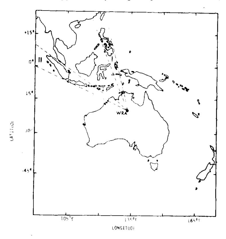
Figure l. Location of theWRAseismicarraywithrespecttoeatthquakeregionsfromwhich events have been used in this study.

Re{ion l: Banda Sea - Halmahera Philippines ilands - Taiwan

Region ll : Sunda arc islands

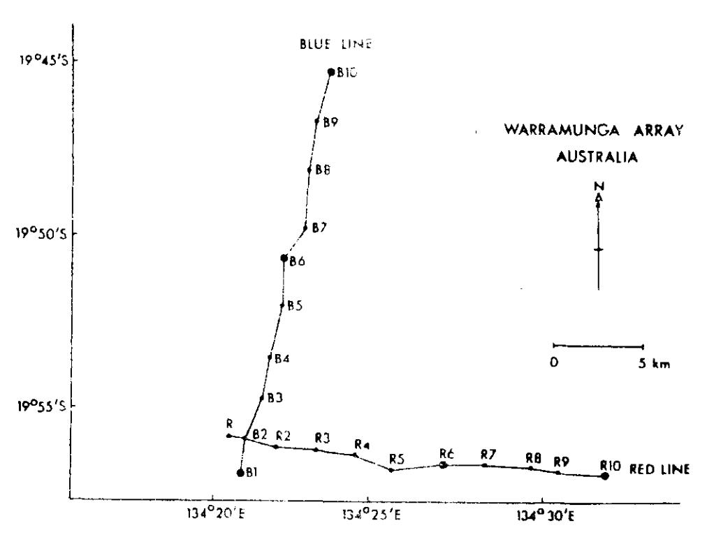
Figure 2. Configuration of the Warramunga Seismic Array. Larger dots contain three component short period instruments.

In 1978, 5 sets of horizontal short period seismometers were installed at station R6, R10, B1, B6, B10. Signals from each seismometer are radio-telemetered to a central recording station and were originally recorded, simultaneously with a time code, on to 24-track FM magnetic tape. In 1978 the primary recording system was changed to a digital recording system and the analog FM tape drive was at this time relegated to providing a back up. For this study records from both vertical and horizontal components and both FM and digital tapes have been used. Output samples of the individual channels are presented in Figure 3.

Many extensive studies using the WRA data have been carried out by Muirhead (1968). King (1974). Ram Datt (1977). Clements (1980). These studies include the enhancements of 3/N by employing processing methods in both the time and frequency. Inmains and the application of several methods of direct slowness calculations. All these processes have their applications and have produced important contributions to the scady of the structure of the earth's interior.

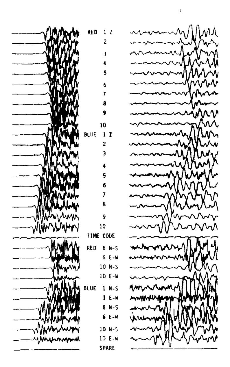
Figure 3. Records of the individual channels of event L1L518 from the Banda Sea region. The P and S records have different normalization scales.

PDE data: 17 Aug. 1979 20h 19 min 36.2 sec 4.372 S 127.270 E ; h = 266 km , Mb = 5.5 Dist. = \(16.72^{\circ}\)

This study is the continuation of that of Muirhead and Ram Datt (1976) and in some cases show better phase resolution especially when the noise level is high.

The N-th root processing technique

With an aperture of about 22 km, the WRA array is small compared with the distance between the source and the array for all except close events. Most arrivals can therefore be considered as plane waves, which implies that they sweep the array with a single apparent velocity and a single direction (azimuth). The azimuth of each event is determined using spherical geometry rule, with the source location given by either ISC (International Seismological Commissions) or PDE (Preliminary Determination of Epicentre).

If \((X_j, Y_j)\) is the location of the j-th sensor, the arrival time relative to the origin of the coordinate system for a plane wave with apparent velocity \(V_a\) and azimuth \(\alpha\) is (see Figure 4)

relative arrival time (time-delay) at \(j^{th}\) sensor: \(t_j = \frac{-r_j \cos{(\alpha - \theta_j)}}{V_2}\)

Figure 4. Time delay as a function of azimuth (\(\alpha\)), apparent velocity (\(V_a\)), and the sensor coordinates.

α is measured clockwise from North (N) to the epicentral direction vector.

\(r_j\) is the radial distance of the \(j^{th}\) sensor can be expressed in cartesian coordinates:

\[r_i = (X_i^2 + Y_i^2)^{1/2}\]

\[tj = \frac{r_j \cos(\alpha - \theta_j)}{v_a}\]

This relative time arrival is also called time delay. The apparent velocity is assumed and the azimuth is known, so the individual sensor channel delay can be taken from its observed arrival time before forming multi channel stack where the N-th root technique is applied. This method (N-th root) is introduced to provide a new method of reducing the effect of non-Gaussian noise which is present in the coda immediately following the first arrival.

After all the channels have been phased (delayed), the N-th root of the wave train magnitudes of each channel are taken, followed by a summing and averaging process. The summed output magnitudes are then raised to the N-th power before forming the TAP (Time Average Product). Even though there is a non-linear distrortion in the signal wave shapes, this technique is a powerful methods of enhancing the S/N, especially for arrival identifications purposes. The maximum TAP for a particular wavelet will determine the right value of assumed \(V_a\), then the measured slowness value (p) will be

\[p = \frac{111.19 \text{ (km/deg)}}{V_{*}(\text{km/sec})} = \text{sec/deg}\]

Mathematically the N-th root technique can be written as follows, if \(f_{ij}\) is the i-th sample of the output of sensor j, the steps of the process are:

1 Take the N-th root of the amplitude of the phased wave train

\[f_{Nij} = |f_{ij}|^{1/N} \operatorname{signum}(f_{ij})\]

2 Determine the average of \(f_{Nij}\) for all sensors, in each arm (Red and Blue) or total.

\[\begin{aligned} & f_{Ni}^{-} \text{ (Red)} = \frac{1}{\text{MR}} \sum_{j=1}^{MR} f_{Nij}; & \text{MR = number of sensors in Red arm} \\ & f_{Ni}^{-} \text{ (Blue)} = \frac{1}{\text{MB}} \sum_{j=1}^{MB} F_{Nij}; & \text{MB = number of sensors in Blue arm} \\ & f_{Ni}^{-} \text{ (total)} = \frac{1}{\text{MR+MB}} \sum_{j=1}^{MR+MB} f_{Nij} \end{aligned}\]

3 Form the N-th root sum by raising \(\overline{f}_{N_t}\) to the N-th power.

\[\begin{split} \hat{f}_{Ni}^{*} & (\text{Red}) = |\overline{f}_{Ni}^{*} (\text{Red})|^{N} \text{ signum } (\overline{f}_{Ni}^{*} (\text{Red})) \\ \hat{f}_{Ni}^{*} & (\text{Blue}) = |\overline{f}_{Ni}^{*} (\text{Blue})|^{N} \text{ signum } (\overline{f}_{Ni}^{*} (\text{Blue})) \\ \hat{f}_{Ni}^{*} & (\text{total}) = |\overline{f}_{Ni}^{*} (\text{total})|^{N} \text{ signum } (\overline{f}_{Ni}^{*} (\text{total})) \end{split}\] 4 The Time Average Product (TAP) is form from the above partial N-th root sums by the relation

\[TAP_i = \hat{f}_{Ni} (Red) \cdot \hat{f}_{Ni} (Blue)\] and the average partial TAP over an s sample window is

\[TAP_{si} = \frac{1}{s} \sum_{k=i-s}^{i} TAP_{k}\]

Muirhead and Ram Datt (1976) determined experimentally that the best value of N for processing WRA data was 4 and this value has been used in this study. It appears to be an appropriate value for enhancing the S/N without excessive distortion of the signal wave shape. The distortion due to this N-th root technique, is not necessary a failing of the technique, but in fact it has advantages. Muirhead and Ram Datt (1976) showed in their experiment on P-wave that in the absence of noise the signal was passed undistorted. This means that those portions of the signal where the S/N level are high are emphasized, which eases the restrictions on both the window length and its position when TAPs are formed to determine slownes measurements. This phenomenon on S-wave data is illustrated in Figure 5 (a through e) which show that wavelets containing noise are converted into a series of narrow sharp impulses. This spiky wave train may not appear aesthetically pleasing to one used to looking seismograms but it can be made to look more like the original signal by smoothing as shown in Figure 5 b.

The advantage of emphasizing portions with large S/N ratios extends to signals that are not correctly phased, with the result that the TAP becomes shaper as a function of slowness or apparent velocity. Consequently, the two unresolved arrival signals with different apparent velocities can be better identified by applying the appropriate velocity when analysing each phase.

This distortion is also sensitive to signal direction (azimuth); and so to obtain a TAP output which is close to the maximum a close approximation to the correct azimuth is required. Previous studies using WRA data (e.g. Ram Datt 1977) have determined that the signal direction obtained either from PDE or ISC source data is close enough to the correct direction when only slowness values are required.

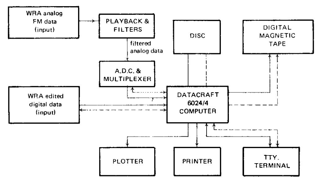
Figure 5. Block diagram of the Data Processing System.

Solid line : flow of information Dashed line : flow of control signals

The processing sequence

WRA data used in this study is available in two formats. The first is analogue data which have been recorded on FM magnetic tapes as continous records. These tapes contain the outputs from the 20 vertical seismometers only and were recorded before the installation of the horizontal instruments. The second are automatically edited digital records which are stored on IBM compatible 9-track tapes. Including timing information, these digital tapes contain the 20 channels of vertical components and 5 channels of S-N and E-W horizontal components.

The chosen events have been retrieved using an analog playback system for the FM tapes and a special plotting program for the digital data. They have been processed by the following sequence:

• digitizing (for the analog data only) and reformatting;
• beam forming using the N-th root technique (as discussed before);
• arrival identification.

After the chosen event has been located, the FM magnetic tape is backed up to a position about 20-30 seconds before it commences. The event is then digitized using a 12-bit A-to-D converter and stored on a temporary disk file. About 500-600 seconds of the event is normally digitized to cover both P and S arrivals. To determine the quality of a record, the first 30 seconds or so of digitized data is plotted out as single-channel records on a calcomp plotter. This plot

allows a visual inspection to determine which seismometers are not working correctly, and these can be masked off in the reformatting stage. Before reformatting, the source parameters, e.g. data source (PDE, ISC), latitude, longitude, origin time, focal depth magnitude and bad channel indicators are typed into a header record programme which computes the expected P and S arrival times based on the J-B travel time curve. This information can be used to select which part of the digitized event and what length will be stored in the reformatted form. Each reformatted event is automatically identified with the digital tape number and the number of the event (or file) on the reformatted digital tape, and this information is printed out for later retrieval purposes. A block diagram of the digitizing-reformatting system is shown in Figure 6.

Because of the noise from the P-wave coda and possible percursors, the first arrival of the S-wave train is not always easy to identify. Besides examining the horizontal component data, a guided trial-and-error method is used. The procedure of this trial-and-error approach are:

• 1 If the P-wave data shows some feature in the travel-time or slowness data, does this same feature exist in the shear wave data?
• 2 The feature of several consecutive arrivals on one trace at a particular distance must be in agreement with those shown by events at nearby distances.
• 3 Excepts as otherwise indicated by possible multiplicity on the travel-time curve, or alternatively the record is noisy, slowness values of arrivals on the same branch must agree within the error of measurements.
• 4 Due to possible errors in source parameters (location and origin time), minor errors in the travel-time have not been considered when constructing composit record sections. In other words, the origin time has been allowed to vary by a few seconds in order to match up corresponding arrivals.

Using these 4 constraints, the procedure of identification of arrivals can be described as follows:

• 1 Using the J-B table for S-wave, the slowness of the first arrival is estimated and the corrected distance is calculated.
• 2 Using the measured slowness values produced by the TAP outputs and a gross shear-wave travel-time curve, the following steps have been followed, starting at the largest distance (in this case about 48 degrees) where the travel-time curve is less complicated and working backwards.
• a) Draw a straight line representing a first-arrival branch of the travel-time curve with almost constant slowness value on graph paper, which has its distance scale on its horizontal axis. This slowness value of this line is initially taken as the measured value of slowness of events at the larger distance range, but can be changed so that the gross S-wave travel time curve is not violated. This reasoning is consistent with the fact that slowness values measured by the

18 SECS.

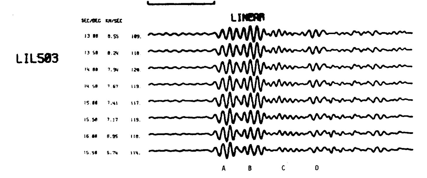
PDE data : 22 Jul 1979 05h 31min 33.3sec 13.858N 124.537E h = 48km M_D = 5.5 Dist = 34.95° Azimuth = 343.20°

Phasing slowness: 13.0 - 16.50 sec/deg with increment 0.5 sec/deg. The above linear-sum traces show four arrival groups A.B.C and D.

Figure 6a. Processed S-wave records of event LIL503

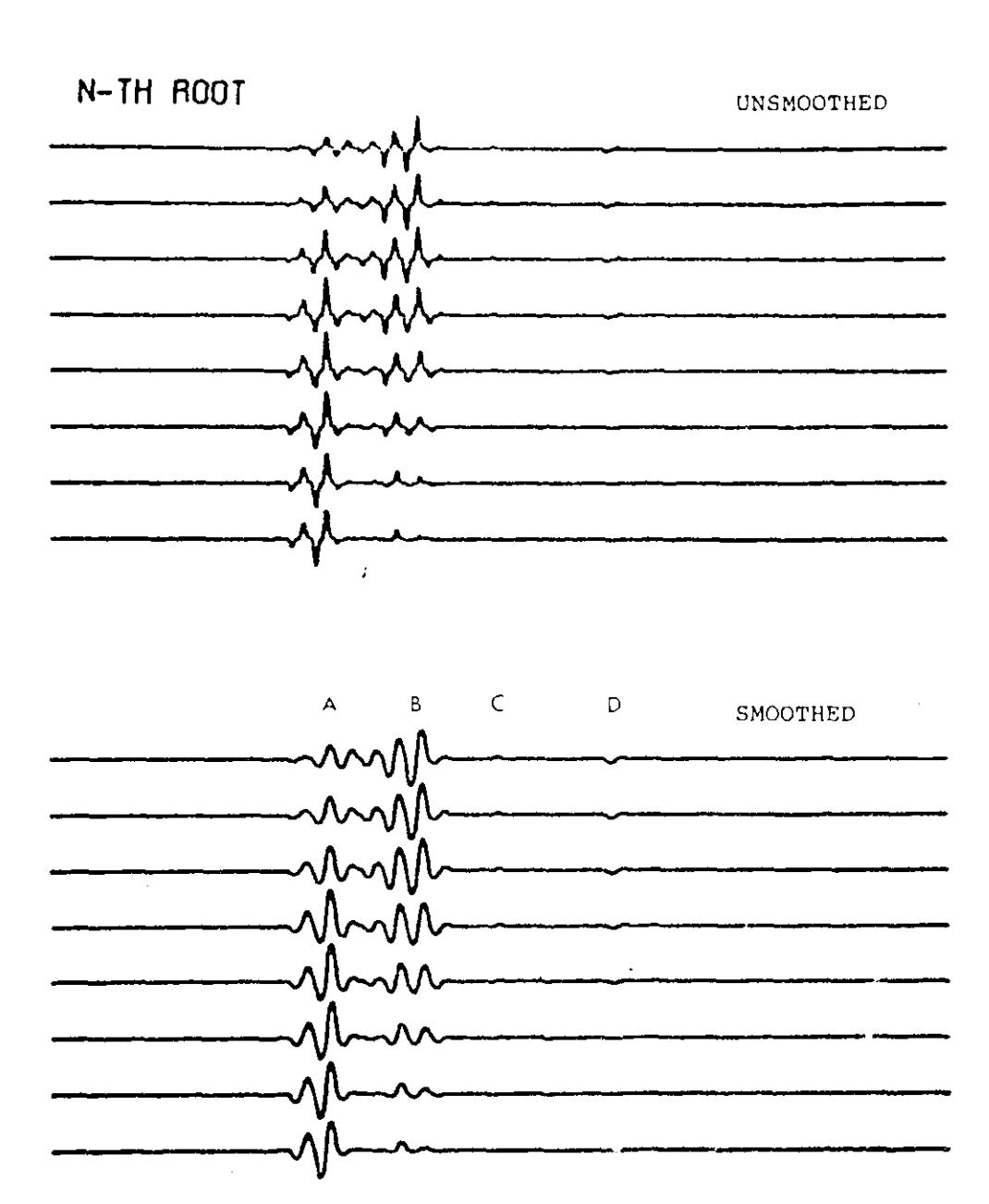
Figure 6b. 4-th-root-sum output phased to the slowness values in Figure 6a The four arrival groups A, B, C, and D are more distinctively resolved

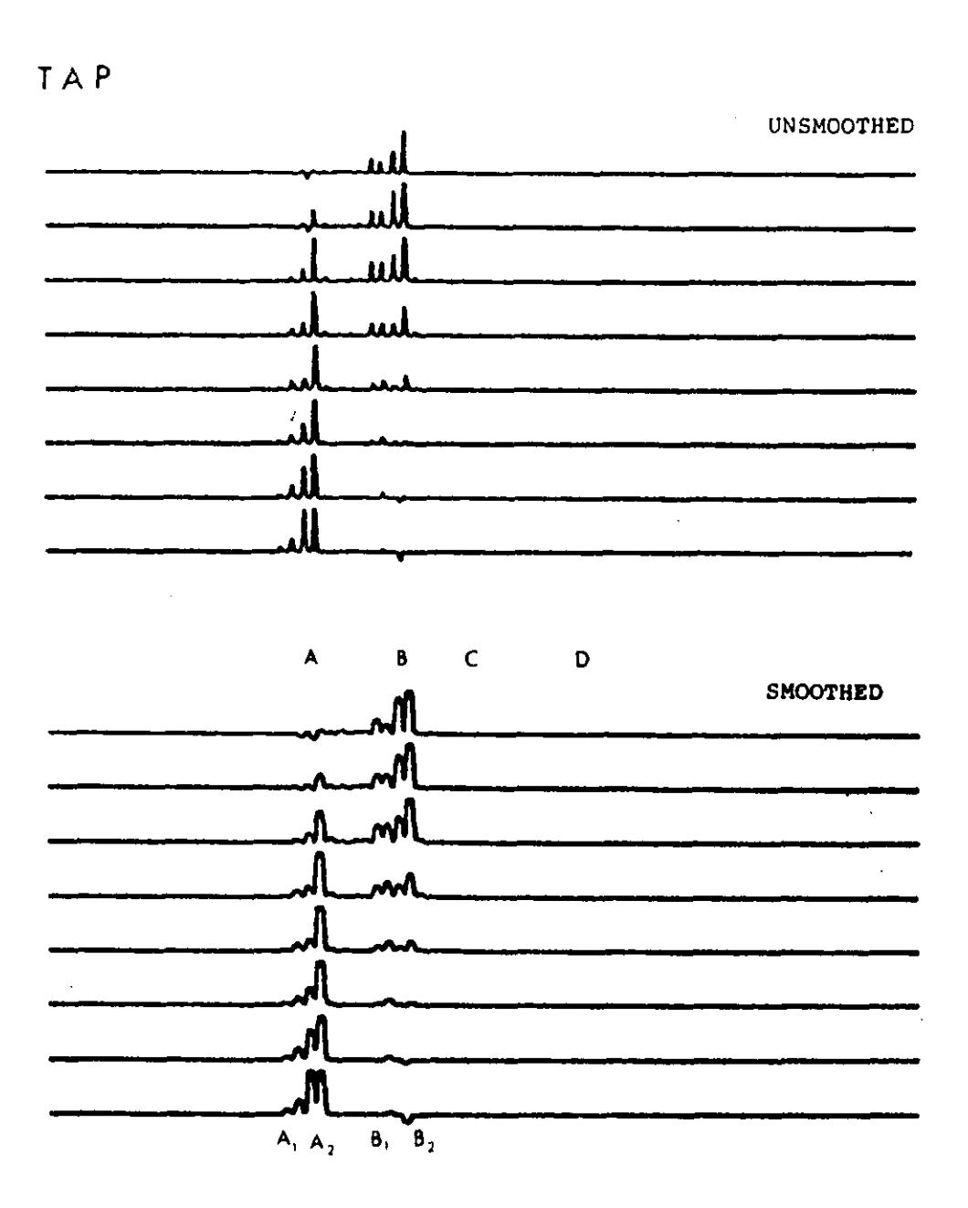
Figuro 6c. TAP (N =4) output phased to the slowness valueJ given in Figure 5a Here il can be seen that A and I may contain more than one signak Ar i3 a phas€ slower than A2; Bl and B;

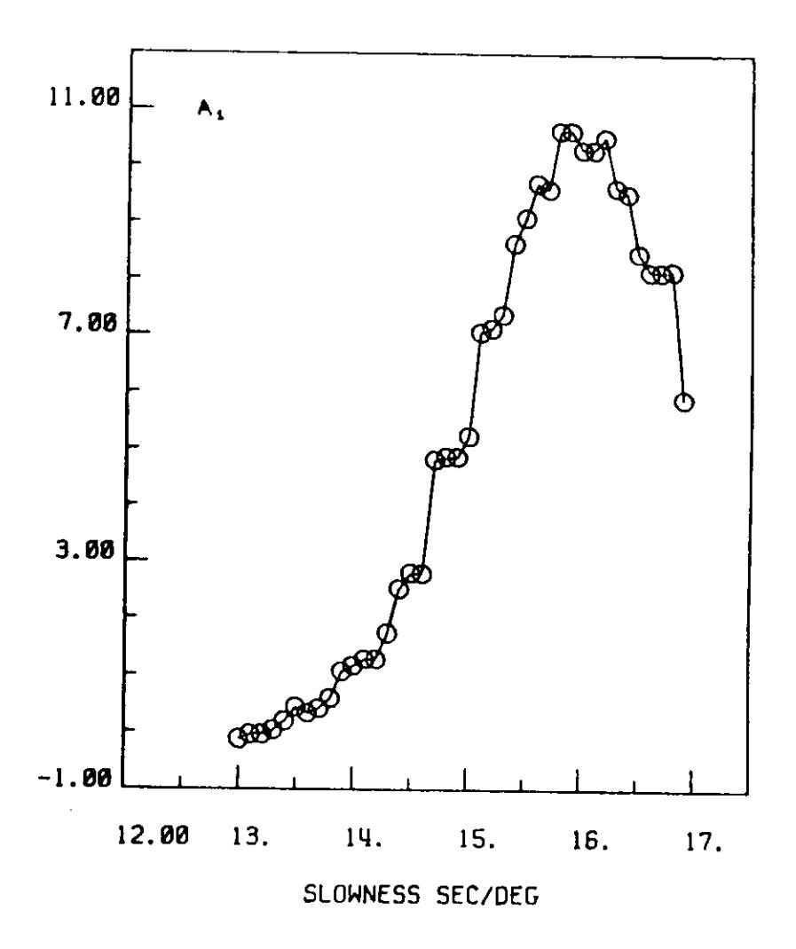
Figure 6d. TAP value of one-second window as a function of slowness, for window contains signal \(\mathbf{A}_1\)

The maximum TAP is at 15-9 sec/deg

array may be offset by structure under the array.

• b) Write down the measured slowness values for the corresponding onset signals on the linear-sum output trace.
• c) Place the trace on the graph paper at the corrected distance and fit the interpreted first onset to the estimated first arrival branch.
• d) Care must be taken with later arrival slowness. They must follow other different straight lines or curves.

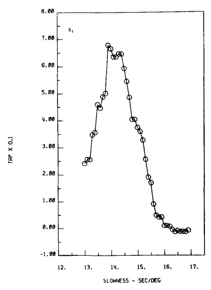
Figure 6e. TAP value of one-second window as a function of slowness, for window contains signal \(\mathsf{B}_1\)

The maximum TAP is at 13.9 sec/deg

• e) Multiplicity of the travel-time is indicated by the convergence of first and intermediate later arrivals to form an intersection. In this case, a second straight line is drawn by referring to the trend shown by the later arrivals. Often, this second straight line is not easily drawn due to possibly more than one multiplicity found in short distance range or uncertainty of the distance of the cross over point (intersection point).
• 3 Continue the steps in 2 until all available output traces cover all corresponding distances, adjusting the straight lines or trace position as necessary to

4 After the final matched configuration has been met, all slowness values are recorder as the measured slowness values for their corresponding travel-time branches, either first or later arrivals. Further more, the shape of the first-arrival travel-time is also obtained.

The phases identified by this procedure must all be identified as S phases. This requires that other phases which occur in the S-wave train must also be identified, especially the one which can disturb the first S arrival as a precursor or immediately after the first S onset. The above mentioned phases are S-to-P conversion (Sp) at the Moho. PcS and ScP (both are the reflected phases from the mantle-core boundary), and PS (reflected phases from the earth's surface). A small computer program using geometrical ray tracing theory has been developed to calculate their travel times to see where they will arrive in the S-wave train at a particular distance.

Some results on first-arrival slowness measurements

Some corrections must be applied to the measured slowness determination to obtain more representative values of \(dT/d\Delta\) versus distance (\(\Delta\)). The requirement for these corrections exist because of different focal depth and local structure under the array. The focal depth correction arises because rays from deep events at a certain distance follow the same path and thus have the slowness value as those from shallow events at a greater distance. The procedure adopted in this study for providing a common base is to project rays from deeper events to a surface focus and thus obtain a corrected distance. A small computer program is used to calculate these corrections using focal depth and slowness value as inputs by applying travel-time (T) and distance (\(\Delta\)) equations described by Bullen (1963, p. 111–112). The velocity distribution model for S used for this correction is adopted from P-wave model CAP8 (Hales et al, 1980) divided by 1.785 (Hales and Muirhead, 1980).

To avoid errors due to local structure under the array the events are selected from the sources which are located in a narrow azimuth range, because the seismic rays travel approximately the same path when arriving at the array. The ratio between observed and corrected slowness is less likely to be perturbed in an unknown manner by local structure (Ram Datt and Muirhead, 1976). The results which will be presented here, are selected from sources within an azimuth range (\(341 \pm 8\)) degrees which is along Banda Sea-Halmahera-The Philipphines-Taiwan trend.

Figure 7 shows first arrival slowness data in the distance range of 12.5 to 22.75 degrees. It can be examined statistically that there are four types of slowness

trends likely to be drawn from the data. This indicates that there should be three distinct velocity boundaries in the earth's mantle within the depth ranges penetrated by seismic rays with slowness shown by the data. Further discussion in this matter will be presented in another paper.

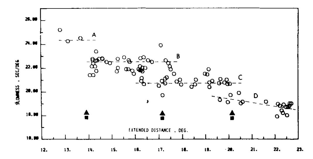
Figure 7. First arrival slowness data in the distance range 12.5 to 22.75 degrees from events from Banda Sea-Halmahera-Philippine islands-Taiwan trend

Three apparent breaks are indicated at distance near 14,17 and 20 degrees. A, B, C, D are four branches of travel-time curve

Conclusions

This experiment concludes that the application of N-th root processing technique on S-wave records produces good result in signal enhancement as in the P-wave processing; in some cases are better. Arrival identification appears to be less difficult, since the distance between signals (phases) along the trace is wider, which is easier to resolve. This is also found in indicating breaks on the slowness data.

Acknowledgements

The author would like to thank Dr. K. J. Muirhead from the Research School of Earth Sciences who provided digitizing, reformatting and initial version of N-th root processing programs, and raised encouraging discussions concerning the topics. This research was funded by The Australian National University Ph.D scholarships (1978–1981).