

SARI
Suatu kode saluran digital dengan waktu tercacal yang mempunyai pasangan ez coder-decoder berupa mesin berteadaan terhingga dan in rian waktu akan diteliti. &luran dianggap tanpa daya ingat. Digunakan dua buah ukuran kineda yaitu probabilitas kesalahan dan jarak bebas minimum. Penggunaan jarak bebas minimum lebih ditekankan karena lebih mudah dier"aluasi dibandingkan probabilitas kesalahan. Untuk probabilitas kesalahan saluran yang kecil, jarak itu merupakan indikator yang sangat baik bagi kinerja sistem; ia didefinisikan sebagai jarak Hanming minimum antara dua buah kemungkinan sekuen keluaran yang berupa sekuen keadaan yang unik dengan panjang dan keadaan yang sama, baik di awal maupun di akhir sekuen, Sebuah algoritma untuk rnenghitung jarak antara sekuen keluaran yang sedemikian itu telah pula dikembangkao; algoritma tersebut juEa mampu mengidentifikasi semua pagngan sekuen keluaran itu. Sebuah algoritma lainnya, didasarkan pada sifatsifat encoder sebagai mesin dengan keadaan berhingga. yang mamFu menqtxtn decoder dengan keadaan berhingga, telah pula ditemukan. Akhirnya, setelah ,nenemukan berbagai pasangzn encoderiecoder yang berupa mesin dengan keadaan b€rhingga, sistem komunikasi digital disimulasikan.
* Jwusan Teknik Firika, Institut T€knologi Bandung
I INTRODUCTION
A particular kind of digital communication system has, as its objective, a channel coding. The main idea behird any channel codhg scheme is to add some redundant bits to the information sequence so that it has the capability to combat channel noise; the cost of implementing such a system and the rate of information transmission should also be considered. The channel encoder transforms t}te information sequence-Y into a discrcte encoded sequencesp which is called a codeword, i.e. the information sequence with the additional redundant bits. This discrete encoded sequence nis input to the communication channel which outputs a sequence !. The channel decoder then transforms t}te received sequence C into a binary sequence ! called the estimate information sequence. Ideally, J will be a delayed replica of the information sequence.,( although the noise may cause some decoding erron. This is the type of digita.l communication system we are concemed with in this paper.
Most of the research on the channel codes has been on clases of linear codes. The baric purpose of codes is to correct erron caused by noisy communication channels, and for this purpose linear codes have many practical advantages. However, the clas of non-linear codes is larger than that of linear codes. Consequently, if we want to obtain t]Ie largest possible number of codewords with a given property, we should consider non-linear codes. The intent of this paper is to investigate the class of non-linear finite state codes, i.e. codes generated by non-linear finite state encoders, by analyzing the state transition diagram of the codes, i.e. the topological, rather tlun algebraic, structue. There are two types of channel codes in common use today: block codes and convolutional codes. Block codes were the earliest type of codes to be investigated, and remain the subject of the overwhelming bulk of the coding litemture. On the other hand, the perfomrance of convolutional codes has proved to be equal, or superior, to that of comparable block codes in nearly every type of practical application. This anomaly, wherein convolutional codes arc easy to implement but relatively unstudied, is due largely to the difficulty of analyzing convolutional codes. Note that every convolutional code is a finite state code;however, not every finite state code is a convolutional code. Here we examine the structure of relatively good codes to understand what makes them better than others, i.e. in terms of closed paths that diverge from and remerge with the same state and the input-output labelling. The results we obtain are far from solving the general problem; however, they do contribute to a better understanding of such codes.
Convolutional codes were lirst introduc€d by Elias [] in 1955 as an a.lternative to block codes. The Viterbi algorithm [2] was proposed in 1967 as an altemative to the then existing sequential and threshold decoding techniques. This algorithm is a recunive optimal solution to the problem of estimating the state sequence of discrete time finite-state Markov process in memoryless noise. Mary problems in digital communications can be cast in this form [4].
A complete treatment of convolutional codes, and one of the most enlighlening, first appeared in a seriesof papers by Fomey [5,6]. ln [5] Forney defined a convolutional encoder as any constant linear sequential circuit. The associated code is the set of all output sequences resulting from any set of all input sequences. He emphasized the algebraic structure of the convolutional codes in his first paper. In the second one [6], the topological structure was emphasized. Here, convolutional codes were characterized by a trellis structure. Maximum likelihood decoding was characterized as finding the shortest path through the code trellis; an efficient solution for which is the Viterbi algorithm.
The key concept in the performance analysisofthe Viterbi algorithm is the concept of an eror event. A tlrst time error event occurs when the true state sequence.,! is tirst excluded by the state sequence actrrally chosen by the Viterbi algorithni !. By using this concept, Viterbi [3] derived a bound on the probability of decoding e rror using the Viteriri algorithm for convolutional codes ald memoryless channels. A simple function, the minimum free distance, was found to be a good indicator of the bit error probability performance. The minimum free distance becarne the most inrportant distance measure for convolutional codes. The best achievable minimum free distance for a convolutional code with a given rate and encoder memory has not been determired exactly. Most code constructions for convolutional codes have been done by computer search. This has prevented the construction of good long codes, since most computer search techniques are time consuming and limited to relatively short constraint lengths. Larsen [7], Paaske [8], and Johanesson [9] published results of a computer construction technique for non-catastrophic codes with maximal minimum free distance for rates ll4, ll3, 112,213, and 3/4. Upper and lower bounds on the minimum free distance for the best convolutional code have also been obtained by using a random coding approach by Paaske lUl and Costello I l0] . An efficient algorithm for finding the minimum free distance based on the state transition diagram of the code has been developed by Bahl et al. 1l and modified by Lanen U2l. This algorithm searches through the state transition diagram of the encoder for the minimum free distancet the diagram is considered as a weighted directed graph whose nodes are tlre states of the encoder and whose branches are the allowable state transitions. The use of a bidirectional search made this algorithm considerably more efficient than any previously known algorithm.
Most of the results stated above (except [6,11,12,]) were derived by using the algebraic stnlcture; ir addition, all these results are restdcted to the class of linear codes. Methods to design the best non-linear tirne invariant finite state codes, by using the topological structure, have not been reported to our knowledpe.
To deal with this difficult problem, in section 2 we adopt the model developed by Gaarder and Slepian [l3] . They developed afinite state model for a digital transmission system. Their objective was to hnd a pair of transmitter-receiver finite state machines, which would optimize a given criterion function for source coding. However, we use this model for channel coding rather than source coding. In our context the objective would be to find a pair of encoderdecoder finite state machines, which would guarantee a similar result to that of maximum likelihood decoding. An advantage of this model lies in the fact that this model is powerful for analyzing both linear and non-linear finite state codes.
To judge the system performance we will use two measures: probability of error and minimum free distance. To deal with the first measure, in section 3 we derive a general bound on the bit error probability based upon the error event probability at a particular node; the bit error probability can be approximated by a relatively simple function of a generalized minimum free distance. The bound on bit error probability for convolutional codes is a simplified form of this general bound. This bound leads us to investigate the second performance measure, minimum free distance, in section 4; in particular, we investigate what facton make a finite state encoder have a large minimum free distance. In section 5 we will discuss the catastrophic property; how the catastrophic propedy can be identified from the state transition diagram of the encoder will be our concem. For simplicity we rcshict ourselves to finite state encoders with one closed communicating class. In section 6 we will use a general bidirectional search algorithm to deal with closed paths identification and the minimum free distance calculation. In section 7 the problem treated is the approximation of the Viterbi algorithm by a finite state machine. A general treatment of tlis problem did not exist previously. Based on this approximation we will construct our decoder machine. However, the results cannot be extended to general channels because the path rnetrics are not integers. Finally, two computer simulation results will be shown in section 8; each has rate l/2. Since the number of decoder states grown rapidly only the decoder statcs of the fint example is shown.
2 THE SYSTEM MODEL
Figure I shows the general finite state digital communication system. Therc is a digital source which has statistically independent. identically distributed outputs and a channel encoder and decoder, both of which are time irLvariant finitc state machines. The channel linking them is assumed to bc mernoryless and time invariant. Furthermore, the entire system is discrete and opcrltes in discrete time. That is, all the system variables take values in finite or coLrntirbly infinite sets and changes occur only at fixed instants in tinre.
Thus, at time n the digital source generates an output sequence, say \(X_1, X_2, \ldots\). Here, each \(X_i\) is drawn from a set of source symbols \(X = (1, 2, \ldots, N_X)\). The channel encoder accepts the sequence \(X_1, X_2, X_3, \ldots\) as an input and produces as an output the sequence \(D_1, D_2, D_3, \ldots\) For \(n = 1, 2, 3, \ldots\) the output \(D_n\) at time n takes values from \(\not D = (1, 2, \ldots, N_D)\). We represent the channel encoder as a time invariant finite state machine with \(N_S\) states, i.e. \(\not S = (1, 2, \ldots, N_S)\). Let \(S_n \in \not S\) be the channel encoder state at time n. We write
\[S_{n+1} = \sigma(X_n, S_n) \tag{1}\]
\[D_{n} = \delta(X_{n}, S_{n}) \tag{2}\] where the functions \(\sigma(.,.)\) and \(\delta(.,.)\) constitute a description of the encoder. Obviously these functions can also be described by a transition table or transition diagram.
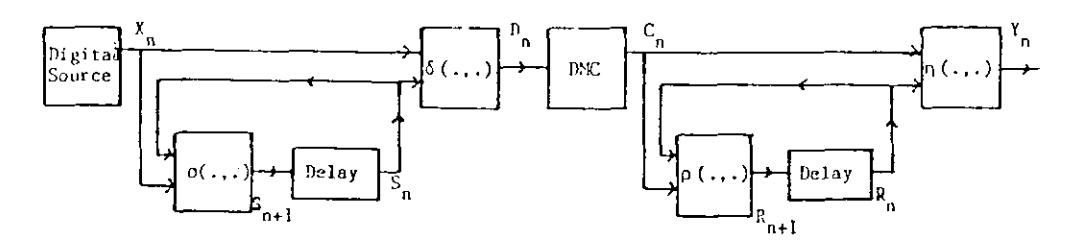
Figure 1. The general finite state digital communication system
The output of the channel encoder, i.e. the encoded message sequence, \(D_1\), \(D_2\), ... is input to the communication channel which outputs the sequence \(C_1\), \(C_2\), ... at a fixed rate. Each \(C_n\) is a noisy version of \(D_n\) and takes values in a given set \(\not = (1, 2, ..., N_C)\).
Similarly, we represent the decoder as a time invariant finite state machine with \(N_{\rm R}\) states, i.e. \(R = (1, 2, 3, ..., N_{\rm R})\). The decoder accepts the sequence \(C_1, C_2, ...\) as an input and produces as its output the sequence \(Y_1, Y_2, ...\) Each \(Y_n\) for n = 1, 2, ... takes values from the set X.
Let \(R_n\) be the decoder state at time n. We write
\[R_{n+1} = \rho \left( C_n, R_n \right) \tag{3}\]
\[Y_{n} = \eta (C_{n}, R_{n}). \tag{4}\]
By defining the channel encoder-decoder as time invariant finite state machines one can prove that:
1. When the \(X_i\) is a sequence of an independent identically distributed random variable, then \((S_n, R_n)\) is a first order Markov chain for a noiseless channel \((C_n = D_n)\) or an additive channel: \(C_n = D_n + N_n\) where + denotes a mod. \(N_C\) addition and \(N_n\) is an independent identically distributed random variable.
2. (rn, S", Rr' y") is a first order Markov chain for a noiseless channel (Cn = Dn) or an additive channel: C = Dn + Nn where + denotes a mod. N6 additlon and N. is a sequence of independent identically distributed random variables. These are shown in Appendix A and B.
We now pose the problem we want to investigate :
Given tlte channel output sequence Ct, Cy, C3,. . ., the channel matrix, the finite state digital channel encoder. find the finite state digital channel decoder such that the output scquence.of this machine, i. e. Y,, Yr, )'r, . . . is an estinrate of Xr, Xt, Xr, . which is close to that of a rnaximumlikelihood decoder.
Maximunl ikelihood dccoding for finite state codes can be realized with the Viterbi algorithn. However, since the number of decoder states have to be finite, a truncated version of the Viterbi algorithm will be used to solve the above problem. In general, the best way to approxintate the Viterbi algorithm with a finite number of the decoder states remains an unresolved problem. We restrict ourselves to a specific case. These difficulties will be more evident in the nex t section.
3 PROBABIUTY OF ERROR
Since both the complexity and the operation of the finite state encoder and decoder depend only on the number of states, code rate, and channel parameters, the block length of the code is irrelevant. Furthermore, the bit eror performance is primarily a function of relative distances among signals, which may be delermined frorn the code state diagram, whose structrue and complexity depend strongly on the constraint length but not on the block length. In addition, block error probability is not a reasonable performance measure, particularly when, as is often the case, an entire message is encoded by the finite state encoder as a single block, whereas in block coding the same message would be encoded into many smaller blocks. Ultimately, the most useful measure is bit error probability Po which is the expected number of bit errors per bit decoded.
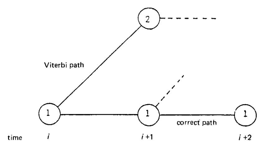
While our ultinate goal is to upper bound P5, we initially consider a more readily determined performance measure, a first error event probability at time i, which we denote P1 (i). Let us recall that first eror event at time i occurs when ths true state sequence,.S, is first excluded at time i by the state sequence actually chosen by the Viterbi algorit hm,f: equivalently one can say that a first error event occurs at time i if the Viterbi path and the corrcct path are difttrent for the first time at tilne i + I. For further analysis it is convenient to expand the state transition diagram of the encoder in the time domain, that is, to represent each time with a separate state diagram;the resulting structure is called a trellis diagram. In the trellis we can now define that the error event occurs at tine I if the Viterbi and thc correct path are the same at time i but they are different at time i + l. frigr.rre 2 shows a situation when a first error event occurs at time I in the trellis. By definition we get:
4(t) = PrIthe Viterbi path and the correct path, in the trellis, are t]re same at time i but different at time i + ll. (5)
Fiqu?e 2 An example of a first error event at time i
Although the Viterbi path and the correct path are different at time i + l, they remerge at some time, at least when the decoder is forced to arrive at a knowtr final state to make the decision. Let these two paths remerge at time i + nr. Since all possible Viterbi paths of length i + ln or more can cause a first error eveitt at time i, the first error event probability at time i, p1 (i), can be overbounded. by the union bound, by the sum of the error probabilities of clch of these paths. Obviously Hq. (5) can be rewritten:
Pt (i) = PrlH { the Vitcrbi parh and the correct path, in the trellis. are the same at time i but different at time I + I andremergeat timei+rn] l. (6) Pi(r) < f,, P, ftn" Viterbi path and thc correct path. in the trellis, are the same at timc I but different at tinle i+ I and remeryeat timel +r?j.
Figure 3 shows some possible Viterbi paths that diverge fronr the correct path at tinre i and renrerye at time i + rn 1or sonte value of rrr, known as tire incorrect subset for time L For this to occur, tlte correct path metric increments over the unnrerged segment, that js over the tintc spalt between i and i + ra. ntust be less

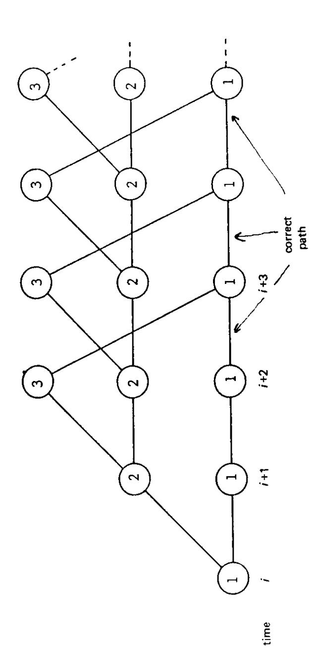
than those of the incorrect path. Let \(\underline{S}\) and \(\underline{\widehat{S}}\) denote the correct and the Viterbi paths, respectively; given that \(\underline{S} = \underline{S}_k\) is the correct path then Eq. (6) can now be rewritten:
\[P_{\mathbf{f}}\left(i \mid \underline{S} = \underline{S}_{\mathbf{k}}\right) \leq \sum_{S_{\mathbf{k}}} \sum_{\epsilon \mid A_{\mathbf{k}i}} Pr\left\{M_{i+m}\left(\widehat{\underline{S}}_{\mathbf{k}}\right) - M_{i}\left(\widehat{\underline{S}}_{\mathbf{k}}\right) > M_{i+m}\left(\underline{S}_{\mathbf{k}}\right) - M_{i}\left(\underline{S}_{\mathbf{k}}\right)\right\}\](7)
where \(M_j(\underline{S})\) is the metric of the \(\underline{S}\) path at time j and \(A_{ki}\) is the incorrect subset of \(\underline{S} = \underline{S}_k\) for time i, that is, all possible incorrect paths that diverge from the correct path \(\underline{S} = \underline{S}_k\) at time i. By noticing that this bound is independent of i, one finds that it holds for all i. Since \(M_{i+m}(\underline{S}_k) - M_i(\underline{S}_k)\) is simply the metric increment of \(\underline{S}_k\) over the time span between i and i+m then the first error event probability at any time, given that \(\underline{S} = \underline{S}_k\) is the correct path, is simply upper-bounded by:
\[P_{\mathbf{f}}(\underline{S} = \underline{S}_{\mathbf{k}}) \leq \underbrace{\widehat{S}_{\mathbf{k}}}_{\mathbf{K}} \underbrace{\sum_{\mathbf{K}} \sum_{\mathbf{K}} Pr[\Delta M(\widehat{\underline{S}}_{\mathbf{k}}, \underline{S}_{\mathbf{k}})]}_{\mathbf{K}}\](8)
where \(\Delta M(\hat{S}_k, \underline{S}_k)\) is the difference between the metric increment of \(\underline{\hat{S}}_k\) and \(\underline{S}_k\) over the unmerged segment, and \(A_k\) is the incorrect subset of \(\underline{S} = \underline{S}_k\). Clearly the first error event at any time is upper-bounded by:
\[P_{\rm f} \leq \sum_{\rm k} Pr[\underline{S} = \underline{S}_{\rm k}] \sum_{\widehat{\underline{S}}_{\rm k}} \sum_{\epsilon A_{\rm k}} Pr[\Delta M(\widehat{\underline{S}}_{\rm k}, \underline{S}_{\rm k})]. \tag{9}\]
The final Viterbi path can diverge and remerge with the correct path any number of times, that is, it can contain any number of error events. Figure 4 shows a situation where multiple error events occur. After the first error event has occurred, the two paths to be compared will both be incorrect paths, one of which will be a previous error event. This is illustrated in Figure 5, where it is assumed that some segments of the correct path \(\underline{S}\) have been excluded for the first time at time i by an incorrect path \(\underline{S}_1\), and assumed that there is another incorrect path \(\underline{S}_2\) that diverges from \(\underline{S}\) at time j. However, since at time j they both have the same metric, then whether some segments of \(\underline{S}\) will be excluded
Figure 4 A situation where multiple error events occur
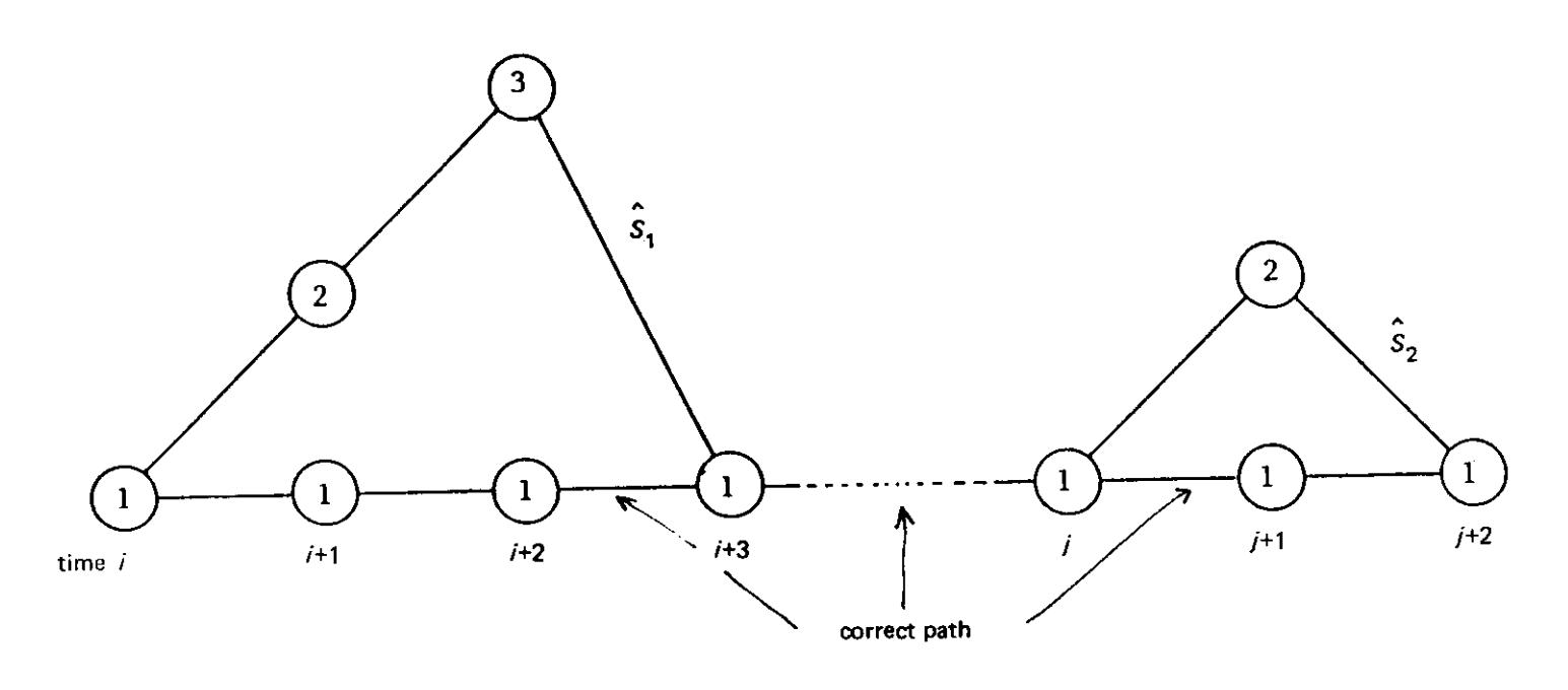
Figure 5 A comparison of two error events
again at time j by \(\widehat{S}_2\) depends only on their metric increment over the time span between j and j+2. If the metric increment over the unmerged segment, that is over the time span between j and j+2, for \(\widehat{S}_2\) exceeds that of some segments of \(\underline{S}\) then \(\underline{S}\) will be excluded by \(\widehat{S}_2\) at time j, and we say the second error event has occurred at time j. Let \(P_2(j)\) denote the probability that some segments of \(\underline{S}\) over the time span between j and j+2 is excluded by \(\widehat{S}_2\) at time j. Now, after the second error event has occurred, the Viterbi path contains \(\widehat{S}_1\), some segments of \(\underline{S}\) over the time span between i+3 and j, and \(\widehat{S}_2\). The probability for this to occur, that is, the error event probability at time j, can be approximated by \(P(E_j) = P_f \times P_2(j)\). Obviously, if \(\underline{S}\) has not been excluded by \(\widehat{S}_1\) at time i then \(P_2(j)\) is simply equal to \(P_f(j)\), a first error event probability at time j. We conclude from this exposition that the error event probability at time j, \(P(E_j)\), is upper-bounded by:
\[P(E_{i}) \leq P_{i}(j) \tag{10}\]
However, since it holds for all time, we will use the error event probability at any time P(E) rather than for a particular time \(P(E_j)\). In addition, we restrict ourselves to finite state codes with one closed communicating class. Let us now evaluate the upper-bound on the error event probability at any time, P(E).
From Eqs. (9) and (10) one can find:
\[P(E) \leq \sum_{\mathbf{k}} Pr[\underline{S} = \underline{S}_{\mathbf{k}}] \sum_{\underline{S}_{\mathbf{k}}} \sum_{\epsilon : A_{\mathbf{k}}} Pr[\Delta M(\underline{S}_{\mathbf{k}}, \underline{S}_{\mathbf{k}})]\] (11)
Let \(\widehat{\underline{D}}_k\) and \(\underline{D}_k\) be the corresponding code sequences of the Viterbi path \(\widehat{\underline{S}}_k\) and the correct path \(\underline{S}_k\), respectively. Each term of the summation over \(A_k\) in (11) is the pairwise error probability for two code sequences over the unmerged segment. For a binary input channel this is readily upper-bounded by a function of the distance between code sequences over this segment. For, if the total Hamming distance between code sequences \(\widehat{\underline{D}}_k\) and \(\underline{D}_k\) (over their unmerged segment) is \(d(\widehat{\underline{D}}_k, \underline{D}_k) = d\), for the binary symmetric channel, the pairwise error probability is bounded by [3]
\[P_{\rm d} \le \exp\left[d \ln \sum_{\ell} (p_0(c) p_{\rm i}(c))^{0.5}\right]\] (12)
where \(P_i(c)\) is the conditional (channel transition) probability of output c given that the input was i(i=0,1). Thus, given that there are a(d) incorrect paths which are at Hamming distance d from the correct path over the unmerged segment, we obtain
\[P(E) \le \sum_{k} Pr\left[\underline{S} = \underline{S}_{k}\right] \sum_{d=d_{\min}}^{\infty} Pr\left[\text{error caused by any one of } a(d(\widehat{\underline{D}}_{k}, \underline{D}_{k}))\right]\]\nincorrect path at distance \(d(\widehat{\underline{D}}_{k}, \underline{D}_{k})\)
\[P(E) \leq \sum_{\mathbf{k}} Pr[\underline{S} = \underline{S}_{\mathbf{k}}] \sum_{d=d_{\min}}^{\infty} a(d(\widehat{\underline{D}}_{\mathbf{k}}, \underline{D}_{\mathbf{k}})) Z^{d(\widehat{\underline{D}}_{\mathbf{k}}, \underline{D}_{\mathbf{k}})}\](13)
\[a(d(\widehat{\underline{D}}_k, \underline{D}_k)) = \sum_{k}, \Delta_{k \, k'}\]
\[\Delta_{k k} = \begin{cases} 1; \underline{D}_{k} - \widehat{\underline{D}}_{k} \neq \underline{D}_{k'} - \widehat{\underline{D}}_{k'}, k' < k \text{ for all } k \\ 0; \text{ otherwise} \end{cases}\] where \(Z = \sum_{c} (p_0(c)p_1(c))^{0.5}\), \(d_{min}\) is the minimum distance of any path from the correct path and \(\Delta_{\mathbf{k}|\mathbf{k}'}\) guarantees that the same configuration on the unmerged segment will not be counted twice by a(d), with this \(P(E|\underline{S}=\underline{0})=P(E)\). Henceforth now we will write \(d(\widehat{\underline{D}}_{\mathbf{k}},\underline{D}_{\mathbf{k}})\) as d.
If the channel transition probability is small, Z will be very small; thus one can
approximate \(\sum_{d=d_{\min}}^{\infty} Z^{d}\) by \(Z^{d_{\min}}\). Consequently the summation over all k is approximately the summation over k such that \(d = d_{min}\). Hence we get
\[P(E) \sim \sum_{\mathbf{k}} Pr[\underline{S} = \underline{S}_{\mathbf{k}}] \ a(d_{\min}) Z^{\dim_{\mathbb{N}}} : \widehat{\underline{S}}_{\mathbf{k}}, \underline{S}_{\mathbf{k}} \in A_{\min}\] (14)
where \(A_{\min}\) is the set of all possible \(\widehat{\underline{S}}_k\) and \(\underline{S}_k\) for all k such that \(d = d_{\min}\). Assume that all \(\underline{S}_k\) are equally probable and have length \(\ell\) over the unmerged
segment, then \(Pr\{\underline{S} = \underline{S}_k\} = \frac{1}{2} \ell\). Let \(\ell_{\min}\) be the minimum length of all unmerged segments which produces \(d_{\min}\). We now find:
\[P(E) \le (1/(2^{\ell_{\min}})) a(d_{\min}) Z^{\ell_{\min}}\] (15)
The Viterbi algorithm requires that a final decision on the most probable code path be made by forcing the coder into a known state. However, one can choose any state as the final state. For simplicity we choose the final state equal to the initial state. The distance between the correct and incorrect paths is then simply equal to the distance between two distinct equal length closed paths which we call the free distance and \(d_{\min}\) is the minimum free distance, \(d_{\text{free}}\). Now we get the final form by rewriting the Eq. (15):
\[P(E) \le (1/(2^{\ell_{\min}})) a(d_{\text{free}}) Z^{\text{d} \text{free}}\] (16)
where \(a(d_{\text{free}})\) can be evaluated from \(L_{1, \ell}\) which is the set of all possible closed paths of length \(\ell'\) that begin with and end with I if the minimum distance between closed paths in \(L_{1,\ell'}\) is equal to \(d_{\text{free}}\).
For an illustrative example let the encoder be as shown in Figure 6. Let us choose the initial and final state I equal to state 1. By using the computational results shown in Table 4 we get:
\(L_{1,6} = \{\underline{S}_1, \underline{S}_2, \dots, \underline{S}_{16}\} = \{1333321, 1333221, \dots, 1222212\}\). From Table 5 we find that there are pairs of correct and incorrect paths with the distance over the unmerged segment equal to 3. Clearly the unmerged segment with minimum length will be contained in the following pairs of closed paths:
\[\text{[rumus tidak dapat ditampilkan dengan baik — lihat PDF asli]}\]
But when we look at the ummerged segment it is apparent that there are only three distinct unmerged segments with minimum length \(\ell_{\min} = 2\); (132, 122), (212, 222), and (332, 322); obviously \(a(d_{\text{free}}) = 3\). If the channel crossover probability is p, one finds
\[P(E) \le (1/4) (3) ((p^{0.5} (1-p)^{0.5})^3).\]
For \(p = 10^{-2}\) one can easily get \(P(1) \le 3.0 \times 10^{-4}\).
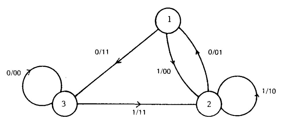
Figure 6 An encoder with three states and \(d_{\text{free}} = 3\)
Turning now to the bit error probability, we note that the expected number of bit errors, caused by any incorrect path which diverges from the correct path, can be bounded by weighting each term of the union bound by the number of bit errors which occurs on that incorrect path. This number is the number of \(\widehat{X}_n \neq X_n\) over the unmerged segments where \(\widehat{X}_n\) and \(X_n\) are the information digits corresponding to the incorrect and correct path, respectively. Thus the bound on the expected number of bit errors caused by an incorrect path is:
\[P_{b} = E[n_{b}] \leq \sum_{k} Pr[\underline{S} = \underline{S}_{k}] \sum_{i=d}^{\infty} i \ a(d, i) \ Z^{d}\] \[\tag{17}\] where a(d, i) is the number of paths diverging from the correct path at distance d and with the number of \(\hat{X}_n \neq X_n\) over the unmerged segments is equal to i. For the same condition we can substitute (16) into (17) and yield:
\[P_{\rm b} \le (1/(2^{\ell_{\rm min}})) \sum_{i} i \, a(d_{\rm free}, i) \, Z^{\rm d_{\rm free}}\] \[\tag{18}\]
For an illustrative example let us use the previous example. It is easy to see that i = 1 for all the unmerged segments and hence \(P_b = P(E) \le 3.0 \times 10^{-4}\). It will be shown in the computational result that for the same encoder and p our simulation get the relative frequency of the error bit which is equal to \(1.0 \times 10^{-4}\)
4 MINIMUM FREE DISTANCE
The most important measure for finite state codes is the minimum free distance \(d_{\text{free}}\). This is largely due to the relation between this distance and the bit error probability according to Eq. (18). In general, the minimum free distance is defined as the minimum Hamming distance between distinct output paths corresponding to state paths of the same length that begin and end with the same state:
\[d_{\text{free}} = \min \left\{ d(\underline{D}', \underline{D}''); \underline{X}' \neq \underline{X}'' \text{ and } \underline{X}', \underline{X}'' \in L \right\}\] \[L = \bigcup_{\mathbf{I}, \mathbf{Q}} L_{\mathbf{I}, \mathbf{Q}}, d(\underline{D}', \underline{D}'') = \sum_{i} |D_{i}' - D_{i}''|\] (19)
where \(\underline{D}'\) and \(\underline{D}''\) are the codewords that correspond to the information sequences \(\underline{X}'\) and \(\underline{X}''\), respectively, i runs over \(\ell\) branches; and \(L_{i,\ell}\) is the set of information sequences produced by traversing closed state paths of length \(\ell\) that diverge from and remerge with the state I.
For a linear code the distance between any two codewords is equal to the weight of another codeword. Hence, for a convolutional code, the minimum free distance is the minimum weight of a codeword produced by a non-zero information sequence. Then for the class of linear codes, Eq. (19) is simplified to:
\[d_{\text{free}} = \min \left( d(\underline{0}, \underline{D}''); \underline{X}'' \neq 0 \text{ and } \underline{X}'' \in L \right)\] \[L = \bigcup_{\varrho} L_{0, \varrho}, \text{ and } d(0, D'') = \sum_{i} |0 - D_{i}''|\] (20)
where \(\underline{D}^{"}\) is the codeword corresponding to the information sequence \(\underline{X}^{"}\); and \(L_{0,\ell}\) is the set of information sequences produced by traversing closed state path of length \(\ell\) that diverge from and remerge with the all-zero state.
Since i in Eq. (19) and (20) runs over \(\ell\) branches, then in terms of graph structure, it seems that an encoder with a greater minimum \(\ell\) should have a bigger minimum free distance. Figure 7 gives an illustrative example of this structural observation. We expect that \(M_1\) will have a bigger minimum free distance than \(M_2\) since the minimum \(\ell\) in \(M_1\) is 3 while in \(M_2\) it is only 2. Those closed state
paths with minimum \(\ell\) in \(M_1\) are \(L_{1,3}\) = (1111, 1241), \(L_{2,3}\) = (2412, 2342), \(L_{3,3}\) = (3333, 3423), and \(L_{4,3}\) = (4124, 4234) while those closed state paths with minimum \(\ell\) in \(M_2\) are \(L_{1,2}\) = (111, 121) and \(L_{2,2}\) = (222, 212).
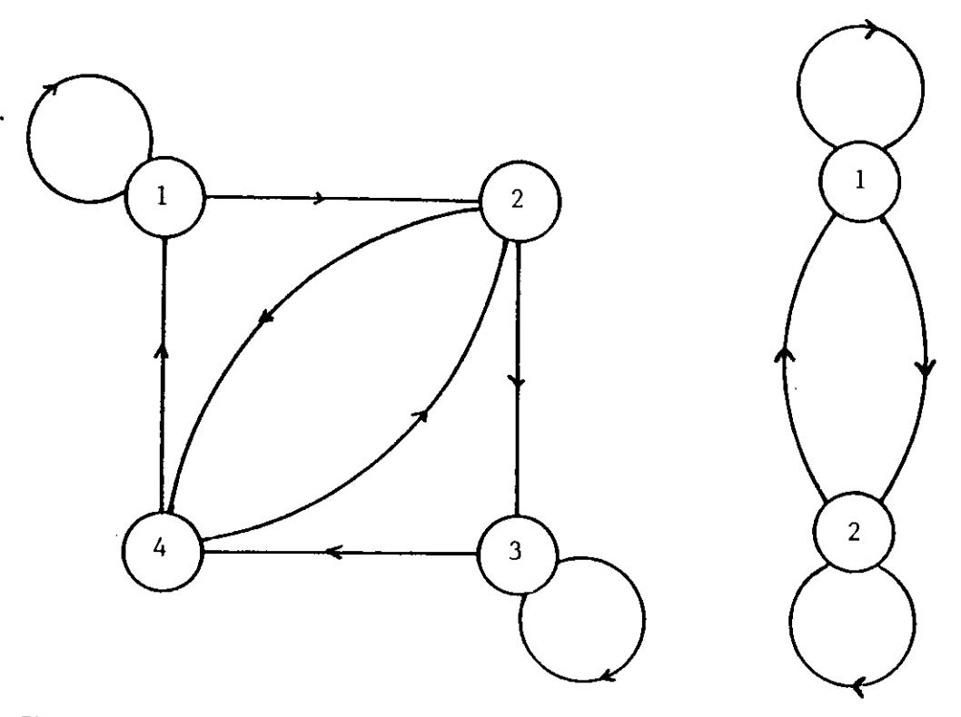
Figure 7 Two encoders with different minimum lengths of closed paths
However, maximum minimum \(\ell\) is not the only condition to ensure a good encoder in terms of its graph. Even an encoder, say \(M_1\), with its minimum \(\ell\) is greater than that of \(M_2\), say, may result in a smaller minimum free distance if there are more branches incommon to the closed state paths in \(L_{1,\ell}\) for \(M_1\) than for \(M_2\). Figure 8 will clarify this immediately.
The encoder \(M_1\) has the minimum \(\ell\) equal to 4 while in \(M_2\) it is only 3. Those sets of closed state paths with \(\ell\) equal to 4 in \(M_1\) are \(L_{1,4}=(11111,12341)\), \(L_{2,4}=(22222,23412), L_{3,4}=(33333,34123),\) and \(L_{4,4}=(44444,41234);\) and for \(M_2\) those sets of closed state paths with minimum \(\ell=3\) are \(L_{1,3}=(1111,1241), L_{2,3}=(2412,2342), L_{3,3}=(3333,3423),\) and \(L_{4,3}=(4124,4234).\) But there are many branches incommon for the longer pairs of closed state paths in \(M_1\). Let us examine a set of closed state paths, with length 5, that diverges from and remerges with state 1, that is \(L_{1,5}=(112341,122341).\) It is clear that there are three branches, out of 5, coincide in \(L_{1,5}\) of \(M_1\) and this certainly

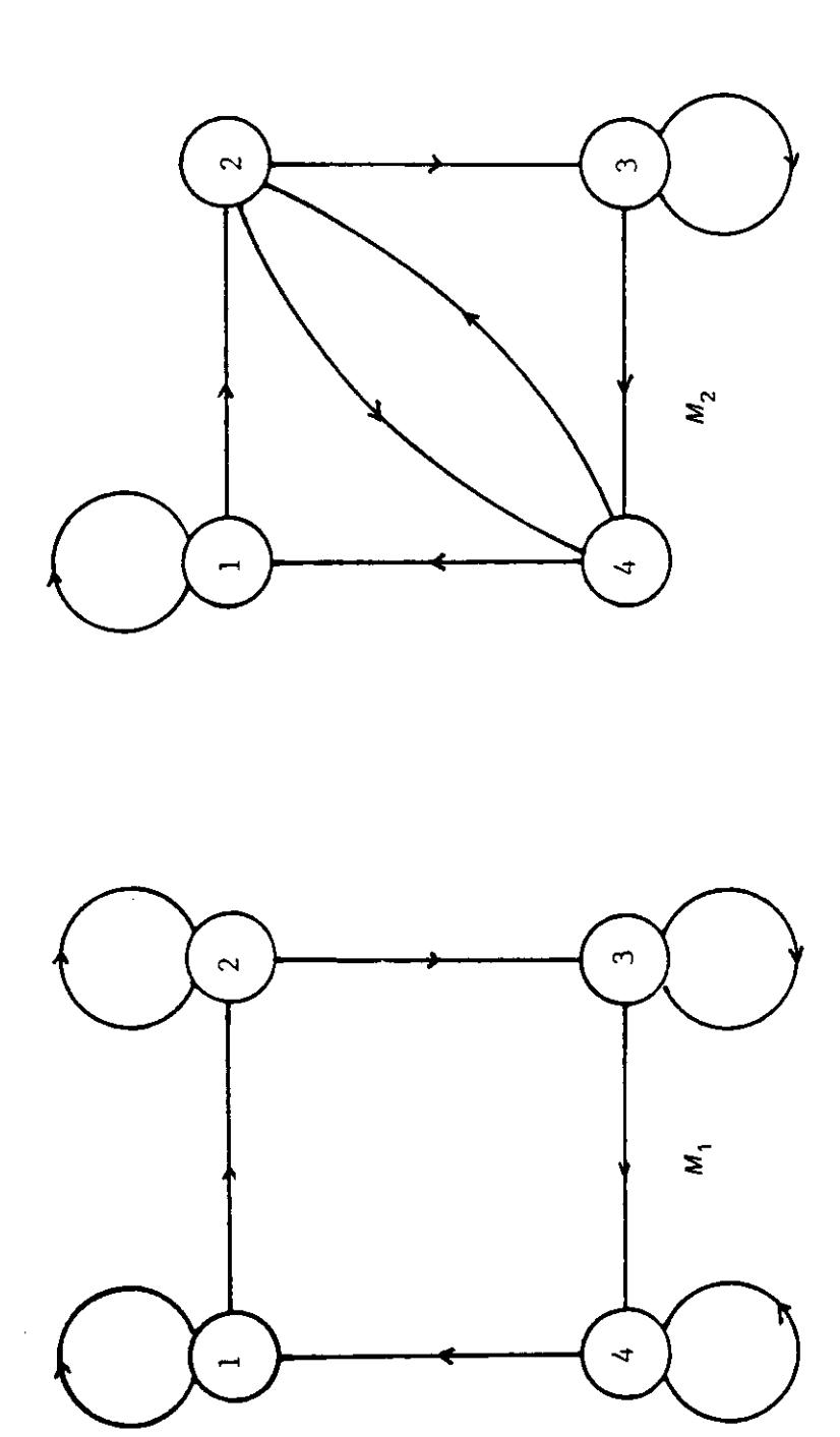
reduces the minimum free distance. This circumstance does not occur in \(M_2\) so that one can expect that \(M_2\) will have a bigger minimum free distance than \(M_1\). However, the largest value of \(\ell\) needed to ensure that one encoder is better than another is still unresolved.
A good labelling should produce maximum minimum free distance while not allowing catastrophic properties; in addition, it also could lead back to the initial state for a fixed input sequence. For a linear finite state encoder (with the all zero state as the initial state) the all zero input leads back to the initial state. So obviously given a good graph with a large minimum \(\ell\) and a minimum number of branches coinciding in \(L_{1,\hat{\chi}}\) another problem remains: the labelling of the branches.
The task of finding methods to design optimal and practical encoders in terms of the state transition diagram appears to be inherently very difficult. Here we provide a computer program to enumerate and identify all closed paths, and having found these closed paths the distances will be calculated for a given encoder. All details of this graph enumerator will be discussed in the next section.
5 CATASTROPHIC PROPERTY
A finite state encoder is catastrophic if a finite number of channel errors cause an infinite number of decoding errors. This undesirable circumstance may happen if there are at least two infinite information sequences \(\underline{X}\) and \(\underline{X}'\) that can be encoded into \(\underline{D}\) and \(\underline{D}'\), respectively, such that
\[d(\underline{D}, \underline{D}') \le \infty \text{ an } d(X, X') = \infty\] (21)
where \(d(\underline{Y}, \underline{Z})\) denotes the Hamming distance between \(\underline{Y}\) and \(\underline{Z}\). If the channel noise changes \(\underline{D}'\) into \(\underline{D}\), by simply changing a finite number of digits of \(\underline{D}'\), then \(\underline{X}'\) will be estimated as \(\underline{X}\) that is infinitely distant from \(\underline{X}'\).
For a linear code it is well known that the state transition diagram of a catastrophic code contains a loop of zero weight other than the self-loop around the all zero state. An example of a linear catastrophic encoder in terms of its state transition diagram is shown in Figure 9. The state transition diagram in Figure 9 contains two cycles, i. e. 00 00 and 11 11, that are generated by different input sequences but have the same output sequences. This certainly will produce catastrophic codes. The following example will clarify this catastrophic property. Let \(\underline{X} = 000000 \dots\) and so \(\underline{D} = 000000000 \dots\) Obviously \(\underline{X}' = 0111111 \dots\) with \(\underline{D}' = 001101000000000 \dots\) in which \(d(D, D') < \infty\) for \(d(\underline{X}, \underline{X}') = \infty\). Consequently, if the channel noise changes the three non zero digits of \(\underline{D}'\) then \(\underline{X}'\) will be estimated as \(\underline{X}\) that is infinitely distant from \(\underline{X}'\). Hence this is a catastrophic code.
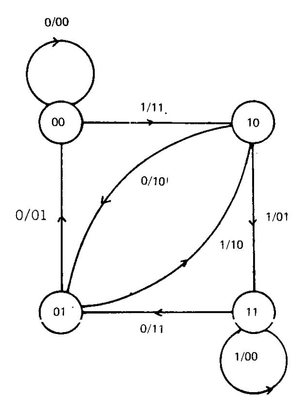
Figure 9 An example of a linear catastrophic finite state encoder with four states
Figure 10 shows an example of a non-linear finite state encoder, in terms of the state transition diagram, that will produce a catastrophic code. The state transition diagram in Figure 10 contains two cycles, i. e. 11 and 232, that are generated by different input sequences but have the same output sequences. This is an obvious catastrophic encoder. The following simple example will clarify this catastrophic property. Let \(\underline{X} = 11010101010...\) and so \(\underline{D} = 111000000...\) Clearly there is \(\underline{X}' = 0000...\) with \(\underline{D}' = 000000...\) has \(d(\underline{D}, \underline{D}') < \infty\) for \(d(\underline{X}, \underline{X}') = \infty\). Hence this is a catastrophic code.
From the above observations one can conclude that in the state transition diagram of a finite state encoder with one closed communicating class Eq. (21) will be satisfied if there are at least two cycles generated by two different input sequences that generate exactly the same output sequence when the cycle repeats forever.
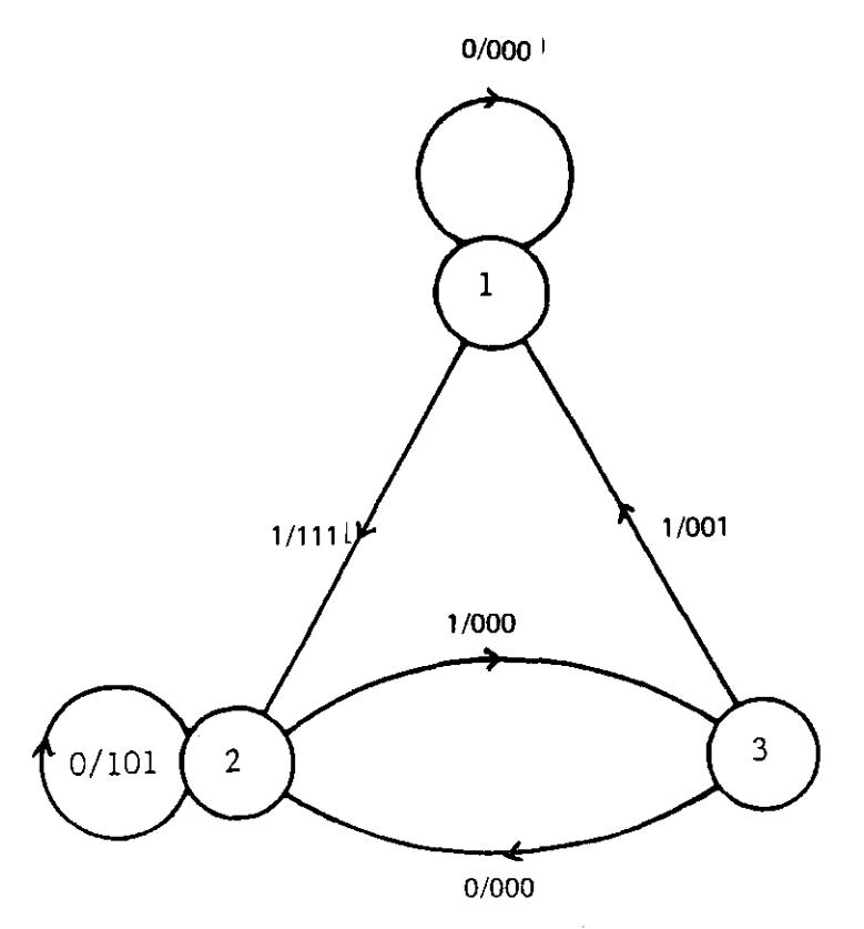
Figure l0 An example of a non-linear catastrophic finite state encoder with three states
6 CLOSED PATH IDENTIFICATION AND d6"" CALCULATION
A comparison of the performance of encoders with the same minimum free distance d1,"" can be obtained by calculating the number of pairs of closed paths that produce d1*"; the better encoder has ttwer such pairs. To identify these pairs we use a generalizcd bidirectional search. This search algorithn will be based on the firite state eircoder as a directed graph tirat can be visualized as a directed tre e.
Consider a finite state cncodcr M with Ns states as a weighted directed gaphi thc nodes are the N5 states of ,/ and the branches are the allowable state transitions. Thc branches of this graph arc labelled rvith the input,/output pairs accordir]g to l-.q. (3). A closed path of lengtir ! that divergcs lronr alld rer')]erges with node I can be visualizcd as a rooted directcd trec with I levels and the temrinal node .qual to the root I, i. c. thc node at le'vel 0. ti.{ = (0. I ) then thjs tree is a binary rooted dircct!'d trce aud therc will bc 2x paths fron thc root to the 2t terminal nodes. Hcnceforth wc considcr otrly binary X. To identify all closed paths of length Q that diverge fronr and renrergc with state I the search
should be conducted on those \(2^{\ell}\) paths that have terminal nodes equal to I at level \(\ell\). Computationally all \(\sum_{i=0}^{\ell} 2^i = 2^{\ell+1} - 1\) nodes should be stored in the memory.
To reduce the number of nodes stored the closed paths are searched from two directions; forward (F) and backward (B). This reduces the number of nodes
stored to \(\sum_{i=0}^{Q/2} 2^{i+1} = 2(2^{(Q/2)+1}-1)\) if the length of the F path is equal to the length of the B path. If \(\ell\) is odd, we choose \(\ell_1 = \lfloor \ell/2 \rfloor + 1\) as the length of the F path, where \(\lfloor y \rfloor\) is the greatest integer smaller than or equal to y, and hence \(\ell_2 = \ell - \ell_1\) is the length of the B path. The closed paths can be determined by merging all F paths and B paths.
An \(F_{\rm I}\) path is defined as a path starting with node I with all arrows pointing in the forward direction. Since the input is binary, there are \(2^i\) paths of length i branches with the same initial node I. The \(F_{\rm I}\) path obviously can be visualized as binary rooted tree with I as the root. Figure 11 shows this observation.
Let \(F_{I,i}\) be the set of all forward paths of length i branches whose initial node is I:
\[F_{1,i} = \{ \underline{f}_j; j = 1, 2, \dots, 2^i \}\] (22)
where each \(f_j\) path is a sequence of states \(f_j = f_{j0} = f_{j0}\), \(f_{j1}\), ..., \(f_{ji}\) and \(f_{jk} = \sigma(x, f_{j(k-1)})\) for some x. Obviously \(f_{j0} = I\) for all j.
Let \(H_{1,i}\) be the set of terminal nodes of all F paths of length i whose initial node is 1. Since each branch represents only allowable state transitions, we can write:
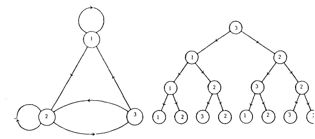
Figure 11. A binary encoder M with its \(F_3\) path that is a binary rooted directed tree
\[H_{\mathbf{I},\mathbf{i}} = \{ \sigma(h_{\mathbf{j}(\mathbf{i}-1)}, k'); k' \in X, h_{\mathbf{j}(\mathbf{i}-1)} \in \$, \ j = 1, 2, \dots, 2^{(\mathbf{i}-1)} \}\] (23)
Obviously for i = 1 we can write \(H_{I,1} = (\sigma(I,0), \sigma(I,1))\).
Without loss of generality, and in a computationally simple manner, we generate \(H_{\mathrm{L},\mathrm{i}}\) as follows:
\[\text{[rumus tidak dapat ditampilkan dengan baik — lihat PDF asli]}\] (24)
This equation implies that the left branches at level i are produced by the input 0 to the nodes at i-1 while the right branches are produced by the input 1. Thus we can generate all the elements of \(H_{1}, \ell_{1}\) recursively from the Eq. (24) for \(i = 1, 2, \ldots, \ell_{1}\).
The next problem is to recover \(F_{\mathbf{I},\ell_1}\) from the elements of \(H_{\mathbf{I},\ell_1}\). Recall that \(f_{\mathbf{j}} \in F_{\mathbf{I},\mathbf{i}}\) has been defined such that \(f_{\mathbf{j}i} \in H_{\mathbf{I},\mathbf{i}}\) for \(i=1,2,\ldots,\ell_1\). Hence the problem of recovering \(F_{\mathbf{I},\ell_1}\) is the same as the problem of choosing the element of \(H_{\mathbf{I},\mathbf{i}}\) to which \(f_{\mathbf{j}i}\) is equal to for all i and i. Since \(H_{\mathbf{I},\mathbf{i}}\) has been generated according to Eq. (24) then this problem can be solved very easily by defining the counting function that in fact serves as a pointer:
Tf
\[K(j,m) = [(j+2^{(i-m)}-1)/2^{(i-m)}]\] (25)
then
\[f_{\rm jm} = h_{\rm Km} \tag{26}\] where
\(h_{\mathrm{Km}} \in H_{\mathrm{I},\mathrm{m}} \text{ and } H_{\mathrm{I},0} = \{1\}\)
[y] = the greatest integer smaller than or equal to y
\[j = 1, 2, \dots, 2^{i}\]
\[m = 0,1,\ldots,i\]
\[i = 1, 2, \ldots, \ell_1\]
Hence \(E_q\). (26) defines \(F_{I,\ell_1} = \{f_j; j=1,2,\ldots,2^{\ell_1}\}\). Note that \(F_{I,\ell_1}\) can also be generated by considering input sequences to the state I as a binary number. Example: Consider the finite state encoder M of Figure 6. Let \(\ell_1 = 3\) and I = 3. Suppose we want to recover \(f_1 = f_{10}f_{11}, f_{12}, f_{13}\). From (22) and (23) we get \(H_{3,1} = \{h_{11},h_{21}\} = \{1,2\}; H_{3,2} = \{h_{12},h_{22},h_{32},h_{42}\} = \{1,2,2,3\}\) and
\(H_{3,3} = \{h_{13}, h_{23}, h_{33}, h_{43}, h_{53}, h_{63}, h_{73}, h_{83}\} = \{1, 2, 2, 3, 2, 3, 1, 2\}\). From (25) we get K(1,0) = K(1,1) = K(1,2) = K(1,3) = 1 and from (26) yields \(f_{10} = h_{10} = 3\); \(f_{11} = h_{11} = 1\); \(f_{12} = h_{12} = 1\) and \(f_{13} = h_{13} = 1\). Hence \(f_{13} = 1\). Analogously we can find all \(f_{13} = 1\), \(f_{13} = 1\).
Define a \(B_{\rm I}\) (backward) path as one starting with I and with all arrows pointing to the backward direction. Unlike an \(F_{\rm I}\) path, the \(B_{\rm I}\) path cannot be visualized as a binary tree because there may be states that can be reached only through a single branch or through more than two branches. Figure 12 will clarify this observation. State 3 has only one predocessor-state 2; state 2 has all three states as predecessors. Clearly \(B_3\) cannot be visualized as a binary rooted directed tree. The treatment of \(B_{\rm I}\) paths is more complicated than that of \(F_{\rm I}\) paths. In a convolutional code, the degree of branches in and out of each state is exactly two. Consequently the \(F_{\rm I}\) and \(B_{\rm I}\) paths in the convolutional codes can be visualized as a binary directed tree; obviously the closed path analysis in a linear class is easier than in a non-linear class of finite state codes.
Let \(G_{I,i}\) be the set of terminal nodes of all \(B_I\) paths of length i whose initial node is I:
\[G_{I,i} = \{g_{ii}; g_{ii} \in \$, j = 1, 2, \dots, N_{Q}(i)\}\] (27)
The elements of \(G_{1,i}\) can be searched recursively by noticing that all nodes at level n are the next state of all nodes at level n + 1. Since all arrows are pointing to the backward direction:
\[G_{I,i} = \{k; \sigma(k,k') = g_{j(i-1)}, k' \in X, k \in \S, j = 1,2,\dots, N_Q(i-1)\}\] (28)
Obviously \(G_{I,0} = \{I\}\) or \(g_{i0} = I\). \(N_Q(i)\) is defined by the counting function:
\[N_{Q}(i) = \begin{cases} N_{Q}(i-1) & N_{S} & 1\\ \Sigma & \Sigma & \Sigma & \Sigma \\ i=1 & k=1 & k'=0 \end{cases} \Delta(\sigma(k,k') - g_{j(i-1)})\] (29)
where
\[\Delta(y) = \begin{cases} 1 ; y = 0 \\ 0 ; \text{ otherwise} \end{cases}\] and \(N_{\mathcal{O}}(j) = 1\) for \(j \leq 0\).
\(N_{\mathbf{Q}}(\mathbf{i})\) counts the number of terminal nodes of \(B_{\mathbf{I}}\) paths of length \(\mathbf{i}\). This number is obviously equal to the number of \(B_{\mathbf{I}}\) paths of length \(\mathbf{i}\) itself.
Let \(B_{I,i}\) be the set of all backward paths of length i branches whose initial nodes is I:
\[B_{I,j} = \{ \underline{b}_j : j = 1, 2, \dots, N_Q(i) \}\] (30)
Associated with each path of \(b_j\) is a sequence of states \(\underline{b}_j = b_{j0}, bj_1, \ldots, b_{ji}\) arranged in the reverse manner such that \(b_{jm} \in G_{1,(i-m)}\) for \(m = 0,1,\ldots,i\).
Since the elements of \(G_{I,i}\) for all i can be generated recursively according to Eq. (28), then the problem of recovering all backward paths \(\underline{b}_{j}\) is the same as the problem of choosing the elements of \(G_{I,(i-m)}\) to which \(b_{jm}\) is equal to for all m and all j. Though the problem is similar to that of recovering the \(\underline{f}_{i}\)
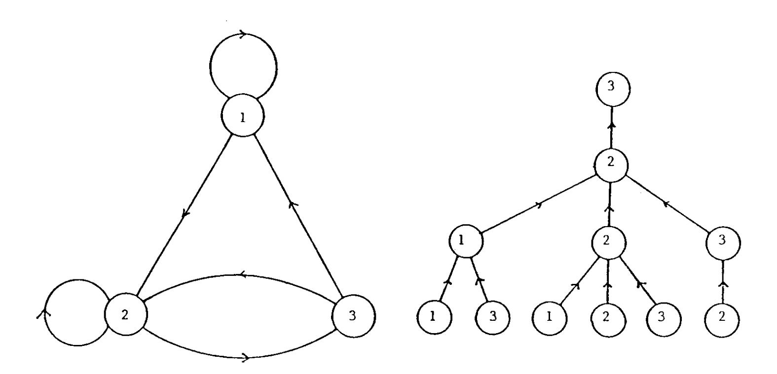
Figure 12 A binary encoder M with its \(B_3\) path that is not a binary rooted directed tree
path, the solution is quite different since the \(B_1\) path cannot be visualized as a binary rooted directed tree. Here we need more counting functions to be used as pointers in \(G_{1,(i-m)}\) to which \(b_{im}\) is equal to where \(i = 1, 2, \ldots, k_2\).
Define the counting function:
\[N_{q}(i,j) = \sum_{k=1}^{N_{S}} \sum_{k'=0}^{1} \Delta (\sigma(k,k') - g_{j(i-1)})\] (31)
\[j = 1,2,...,N_{O}(i-1); i = 1,2,...,\ell_{2}.\]
This counts the number of predecessors of \(g_{j(i-1)}\) for each j. Note that the predecessors of \(g_{j(i-1)}\) are \(g_{ni} \in G_{l,i}\) for all j and \(n = 1, 2, \ldots, N_Q(\ell_2)\). In other words there are \(N_q(i,j)\) elements of \(G_{l,i}\) pointing toward \(g_{j(i-1)}\).
Define another counting function:
\[N_{\mathbf{A}}(k, j(k)) = a_{\mathbf{Nq} \ (k+1, j(k))}\] (32)
\[N_{\mathbf{A}}(\ell_2, j(\ell_2)) = 1 \tag{33}\] where
\[a_{i(k,j(k))} = a_{i(k,j(k))-1} + N_{A}(k+1, c_{i(k,j(k)),j(k)})\] \[c_{i(k,j(k)),j(k)} = \begin{cases} 1; j(k) = 1 \\ \max c_{s(j(k)-1)} + i; \text{ otherwise} \end{cases}\]
\[k = \ell_2 - 1, \ell_2 - 2, \dots, 1\]
\(j(k) = 1, 2, \dots, N_Q(k)\)
\(i(k, j(k)) = 1, 2, \dots, N_Q(k+1, j(k))\)
This counts the number of occurrences of the elements of \(G_{1,k}\) in \(b_{jk}\) of \(\underline{b}_j \in B_{1,i}\) for all k. So the elements of \(B_{1,\hat{k}_2}\) can be described completely by:
\[b_{kj}(\ell_2 - k)) = g_{jk} \tag{34}\] where \(k = 1, 2, ..., \ell_2\); \(j(k) = 1, 2, ..., N_Q(k)\) and
\[i(k, j(k)) = 1, 2, \dots, N_{\mathbf{A}}(k, j(k)).\]
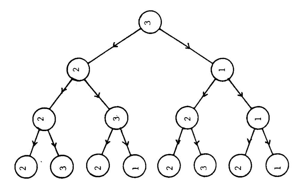
Example: Consider the finite state encoder M of Figure 6. Let \(\ell_2 = 3\) and I = 3. Suppose we want to recover \(\underline{b}_1 = b_{10}, b_{11}, b_{12}, b_{13}\). From (28) and for i = 1 we get \(N_Q(1) = 1\) since \(g_{10} = I = 3\) for all i and \(N_Q(0) = 1\). Then from (26) and (27) we get \(G_{3,1} = \{g_{11}\} = \{2.\}\) If we do the same process for i equal to 2 and 3, then \(N_Q(2) = 3\); \(G_{3,2} = \{g_{12}, g_{22}, g_{32}\} = \{1,2,3\}\) and \(N_Q(3) = 6\); \(G_{3,3} = \{g_{13}, g_{23}, g_{33}, g_{43}, g_{53}, g_{63}\} = \{1,3,1,2,3,2\}\). From (30) we get \(N_Q(1,1) = 1\), \(N_Q(2,1) = 3\), \(N_Q(3,1) = 2\), \(N_Q(3,2) = 3\) and \(N_Q(3,3) = 1\). From (3.12) we find
\(N_{\rm A}(3,1)=N_{\rm A}(3,2)=\ldots=N_{\rm A}(3,6)=1, N_{\rm A}(2,1)=2, N_{\rm A}(2,2)=3, N_{\rm A}(2,3)=1\) and \(N_{\rm A}(1,1)=6\). Now from (3.14) we find that \(b_{12}=b_{22}=b_{32}=\ldots=b_{62}=g_{11}=2,\ b_{11}=b_{21}=g_{12}=1,\ b_{31}=b_{41}=b_{51}=g_{22}=2,\ b_{61}=g_{32}=3,\ b_{10}=g_{13}=1,\ b_{20}=g_{23}=3,\ b_{30}=g_{33}=1,\ b_{40}=g_{43}=2,\ b_{50}=g_{53}=3,\ {\rm and}\ b_{60}=g_{63}=2.\) Since \(b_{11}g_{22}=b_{13}=1=3\) for all j, hence \(b_{11}=b_{11}\) \(b_{11}\) \(b_{12}\) \(b_{13}=1123\).
After having found \(F_{1,\ell_1}\) and \(B_{1,\ell_2}\), one can find all closed paths of length \(\ell = \ell_1 + \ell_2\) that diverge from and remerge with state I by merging the elements of \(F_{1,\ell_1}\) and \(B_{1,\ell_2}\), which is shown in Figure 13, with the following merging rule
Let \(L_{1,\ell}\) be set of all closed paths of length \(\ell\) that diverge from and remerge with state 1:
\[L_{I,\ell} = \{ \underline{S}_i; j = 1, 2, \dots, N_I(\ell) \}\] (35)
where \(N_1(\ell)\) is defined by
\[N_{\mathrm{I}}(\ell) = \sum_{\mathrm{m}} \sum_{\mathrm{k}} (f_{\mathrm{k}} \ell_{\mathrm{I}} - b_{\mathrm{m}0}) \tag{36}\]
Associated with each closed path \(\underline{S}_j\) is a sequence of states \(\underline{S}_j = S_{j0}, S_{j1}, \ldots, S_j\) where \(S_{ji} \in \$\) for all i and all j. Obviously \(S_{j0} = S_j = I\). From the derivation of (25) and (33) it follows that the elements of \(L_{1/2}\) are identified completely by:
\[S_{ji} = \begin{cases} f_{ki}, i = 0, 1, \dots, \ell_1 \\ b_{m(i-\ell_1)}, i = \ell_1 + 1, \ell_1 + 2, \dots, \ell \end{cases}\] (37)
such that
\[f_{\mathbf{k}\,\ell_1} = b_{\mathbf{m}\,0} \tag{38}\] where \(k=1,2,\ldots,2^{\ell_1}\) and \(m=1,2,\ldots,N_Q(\ell_2)\). Hence \(N_I(\ell)\) and \(L_{I,\ell}\) enumerate and identify all closed paths of length \(\ell\) that diverge from and remerge with the state I respectively. The number of closed paths of length \(\ell\) that diverge from and remerge with state I may also be calculated by using the adjacency matrix of the encoder.
Let the adjacency matrix \(M = [m_{ij}]\) of an encoder M be an \(n \times n\) matrix with \(m_{ij}\) defined as:
\[m_{ij} = \begin{cases} 1 ; S_j = \sigma(S_i, X_i) \\ 0; \text{ otherwise} \end{cases}\]
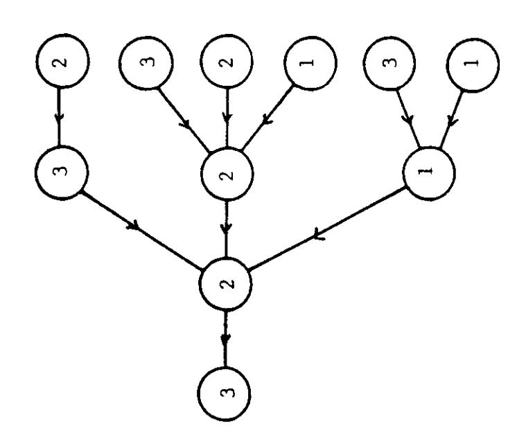
Let \(m_{ij}(\ell)\) be the (i,j) entry of the \(\ell^{th}\) power of the matrix M, then from \(\{21\}\) we get \(N_{I}(\ell) = m_{II}^{(\ell)}\) Now we are ready to calculate the distance between two closed paths.
Consider two closed paths of length \(\ell\), in terms of state sequences, that diverge from and remerge with state I:
\[S_1 = S_{10}, S_{11}, \dots, S_1 \varrho\] (39)
\[\underline{S}_2 = S_{20}, S_{21}, \dots, S_{20}\] (40)
where \(S_{j0} = S_{j\ell} = I\), and \(S_{ji} \in \underline{S}\) for all i and all j. These two closed paths can be described in terms of output label sequences \(\underline{D}_1\) and \(\underline{D}_2\), respectively, as follows:
\[\underline{D}_1 = D_{10}, D_{11}, \dots, D_{1(\hat{X}-1)}\] (41)
\[\underline{D}_2 = D_{20}, D_{21}, \dots, D_{2(k-1)}\] (42)
where \(D_{ji} = \delta(S_{ji}, X_n)\) such that \(\sigma(S_{ji}, X_n) = S_{j(i+1)}\) where \(X_n \in X = \{0,1\}\).
Hence the distance between \(\underline{S}_1\) and \(\underline{S}_2\) is simply:
\[d_{12} = \sum |D_{1i} - D_{2i}|. (43)\]
7 THE DECODER
Consider a path of length \(\alpha\) in a state transition diagram of an encoder of a complete and simple minimal machine \((N_S, N_X, N_D)\). There are \(N_X\) paths of length \(\alpha\) entering the \(N_S\) states for \(\alpha \ge N_S - 1\). There is at least one path of length \(\alpha\) entering each state.
If we apply a truncated version of the Viterbialgorithm, then the number of paths of length \(\alpha\) entering \(N_S\) states can be reduced to exactly \(N_S\) paths where each of them minimizes the metric \(M(\underline{D})\). Obviously the last symbol in each of these paths is unique.
Let \(\underline{S}_{in}^{\alpha}\) be the \(i^{th}\) path of length \(\alpha\) at time n with metric \(M_{in}\) and terminated by the state i. We can write:
\[\underline{S}_{in}^{\alpha} = S_{i(n+\alpha)}, S_{i(n+\alpha-1)}, \dots, S_{in} S_{ij} \in \$ = (1,2,3,\dots,N_S); S_{i(n+\alpha)} = i \ni = 1,2,3,\dots,N_S j = n,n+1,\dots,n+\alpha.\] (44)
This path corresponds to an encoder output sequence of:
\[\underline{D}_{in} = D_{i(n+\alpha-1)}, D_{i(n+\alpha-2)}, \dots, D_{in}\] (45)
yh:t. rq =. 6 (,St,Xj ) such that o(Sij,X, ) = S,rj*, ). W. can search S,in *,, recursrveiy as Io ows:
\[\underline{S}_{j(n+1)}^{\alpha} = r(\underline{S}_{in}^{\alpha}, C_{n+\alpha})\] (46)
where r(.,.) is defined such that:
\[M_{j(n+1)} = \min\{M_{in} - \ln Pr(C_{n+\alpha} | D_{i(n+\alpha)}); D_{i(n+\alpha)} = \delta(S_{i(n+\alpha)}, X_k)\}.\] (47)
Since o(S,,rr*or.{r ) = Siln*o* q y we find
\[\underline{S}_{j(n+1)}^{\alpha} = S_{j(n+\alpha+1)}, S_{i(n+\alpha)}, \dots, S_{i(n+1)}\] (48)
whcreSlln+o+ry =1.
Let,sn = ({;, 6;, . . ., Ifi" ,' )r and the corresponding metric vector
Mn = (Mn, Mrn, .., /r.n,t. A transition from Sn to Jnrl is simply n transition of its components according to Eo. (48). Now we can write the state of the channel decoder at time n as follows: -
\[R_{n} = (\underline{M}_{n-\alpha}, \underline{S}_{n-\alpha})\] or (49)
\[R_{n} = \begin{bmatrix} M_{1(n-\alpha)}, 1, S_{1(n-1)}, \dots, S_{1(n-\alpha)} \\ M_{2(n-\alpha)}, 2, S_{2(n-1)}, \dots, S_{2(n-\alpha)} \\ \dots, \dots, \dots, \dots \\ \dots, \dots, \dots, \dots \\ M_{N_{S}^{(n-\alpha)}}, N_{S}, S_{N_{S}(n-1)}, \dots, S_{N_{S}(n-\alpha)} \end{bmatrix}\] where n ) o. The next state Rn., 1 is just
\[R_{n+1} = (\underline{M}_{n-\alpha+1}, \underline{S}_{n-\alpha+1})\] (51)
Since the decoder states are derived from a truncated version of the Viterbi algorithm, the output of this machine at time n can be computed from the fact that.gn consists of all suwivors with the best metrics. So we first choose fj, so that,44n1 is the smallest component of ,11n, then the output is the input to the encoder machine that causes the transition from S,,n_ o, to Si,n_ o* r,,
\[Y_{\mathbf{n}} = X_{\mathbf{n} - \alpha} \tag{52}\] where M, = min. Mn such that Si(n_o+r) =o(Xn o, Sit. o',);,Mn standS for the components of -Mn. From Eq. (3.32) one can easily notice that the decoding decisions always lag the progrcss of the decoder by an amount equal to the path length d.
It is obvious from Eq- ( I ) and Eq. (49) that Eq(50) will generate more decoder states as n increases; consequently the decoder does not have a finite number of states. This is certainly an undesirable circumstance.
Consider a finite state encoder and a path of length \(\alpha\) in its state transition diagram. Let this encoder have \(N_S\) states. Since the elements of \(\underline{S}_{jn}^{\alpha}\) are drawn from a fixed finite set, the number of possible combinations of the elements of \(\underline{S}_n\), i.e. all paths of length \(\alpha\), is also finite; however, the \(\underline{M}_n\) components make the number of decoder states grow to infinity since each \(M_{in}\) is nondecreasing. Fortunately, the absolute value of the \(\underline{M}_n\) components are not important. The Viterbi algorithm requires only the differences between components of \(\underline{M}_n\). This condition allows us to keep \(\underline{M}_n\) in a fixed range. The finiteness of the decoder state will be based on this property of the Viterbi algorithm.
To maintain the differences between the \(\underline{M}_n\) components fixed while their absolute values grow is achieved by subtracting the smallest component of \(M_n\) from all components of \(\underline{M}_n\). Hence at all times there is at least one component equal to zero. Now, if the metrics between states of the encoder only take integer values, \(\underline{M}_n\) will take only a finite number of values. For the BSC this expectation is fulfilled. In applying the Viterbi algorithm to the BSC, one finds that the algorithm essentially finds the path closest to the received word in Hamming distance.
We can choose any state as the initial state of the encoder and label it as state 1. \(R_0\) is generated by assuming that the decoder receives a sequence of 0's of length \(\alpha\) where \(\alpha \ge N_S - 1\). So we have \(S_{i0} = 1\) for all \(i = 1, 2, \ldots, N_S\). Hence we can write
\[R_{0} = \begin{bmatrix} M_{10}, 1, S_{1(\alpha-1)}, S_{1(\alpha-2)}, \dots, 1 \\ M_{20}, 1, S_{2(\alpha-1)}, S_{2(\alpha-2)}, \dots, 1 \\ \dots, \dots, \dots, \dots, 1 \\ \dots, \dots, \dots, \dots, 1 \\ \dots, \dots, \dots, \dots, 1 \\ \dots, \dots, \dots, \dots, 1 \end{bmatrix}\] \[M_{N_{S}0}, N_{S}, S_{N_{S}(\alpha-1)}, \dots, \dots, 1\] (53)
where \(S_{ij} \in \$ = (1, 2, ..., N_S)\) for \(i = 1, 1, ..., N_S\) and \(j = 1, 2, ..., \alpha - 1\).
Let \(M_{j0}\) be the smallest component of the set \(M_n = \{M_{i0}; i = 1, 2, ..., N_S\}\). Then the Eq. (53); can be rewritten:
\[R_{0} = \begin{bmatrix} M_{10} - M_{j0}, 1, S_{1(\alpha-1)}, S_{1(\alpha-2)}, \dots, 1 \\ M_{20} - M_{j0}, 2, S_{2(\alpha-1)}, S_{2(\alpha-2)}, \dots, 1 \\ \vdots & \vdots, & \ddots, & \vdots \\ 0 & j, S_{j(\alpha-1)}, S_{j(\alpha-2)}, \dots, 1 \\ \vdots & \vdots, & \ddots, & \vdots \\ M_{N_{S}0} - M_{j0}, N_{S}, S_{N_{S}}(\alpha-1), & \dots, 1 \end{bmatrix}\] \[(54)\]
For a BSC with transition probability p < 1/2, the received sequence C is binary and the log-likelihood function becomes
\[\ln Pr(C/D) = d(C,D) \ln(p/(1-p)) + N \ln(1-p)\] (55)
where \(d(\underline{C},\underline{D})\) is the Hamming distance between \(\underline{C}\) and \(\underline{D}\). Since when p is less than 1/2, \(\overline{\ln}(p/(1-p)) < 0\) and \(N \ln(1-p)\) is constant for all \(\underline{D}\), an equivalent maximum likelihood decoder for the BSC chooses \(\underline{D}\) as the codeword that minimizes the Hamming distance
\[d(\underline{C},\underline{D}) = \sum_{i} |C_{i} - D_{i}|. \tag{56}\]
Hence in applying the Viterbi algorithm to the BSC, the metric becomes an integer.
For many of DMC's positive integers can be the metric. The metric \(M(C_i/D_i) = \ln Pr(C_i/D_i)\) can be replaced by \(b_2\) (\(\ln Pr(C_i/D_i) + b_1\)) where \(b_1\) is any real number and \(C_2\) is any positive real number. A path \(\underline{D}\) that maximizes \(\ln Pr(C_i/D_i)\) in fact also maximizes \(b_2\) (\(\ln Pr(C_i/D_i) + b_1\)) and hence the modified metrics can be used without affecting the performance of the Viterbi algorithm.
If \(b_1\) is chosen to make the smallest metric equal to 0, \(b_2\) can then be chosen so that all metrics can be approximated by integers. There are many sets of integer metrics possible for a given DMC, depending on the choice of \(b_2\). The performance of the Viterbi algorithm is now suboptimum due to the modified metrics.
For some transition probabilities such as 1/3, 1/7, etc., even using the modified metrics, we may never have a set of integers as our metrics. From now on we restrict ourselves to the BSC only.
8 COMPUTATIONAL RESULT
Two programs, written in FORTRAN 77, were run on an TSO-IBM 3081 to obtain the results in this section. One program enumerated and identified the closed paths, the minimum free distance, and simulated the communication system while the other generated the finite state decoder.
Two examples will be shown; each has rate 1/2. Since the number of decoder states grows rapidly, only the decoder state of the first example is shown.
EXAMPLE 1
The linear finite state encoder \(M_x\) with two states is chosen because the number of decoder states is small; this makes it possible to show the state transition diagram on one page. Figure 14 shows the encoder while Figure 15 shows the corresponding finite state decoder; state 1 is chosen as the initial state. The decoder states are computationally generated in tabular form; they are shown in Table 1. The enumeration and identification of the closed paths, and the
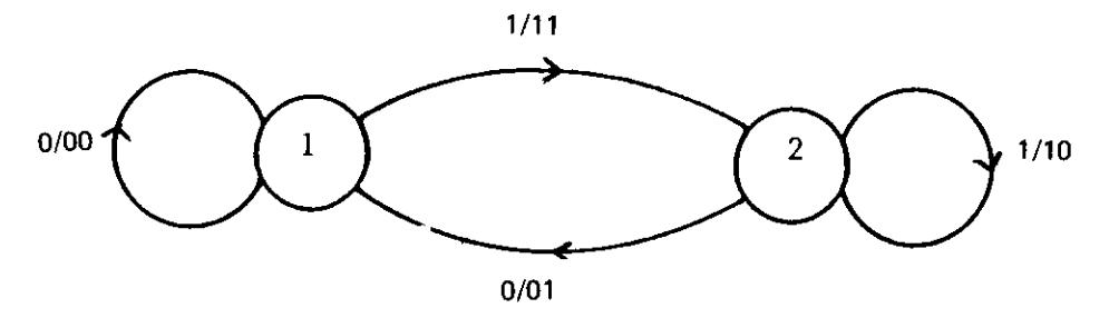
Figure 14 A linear encoder Mx with two states
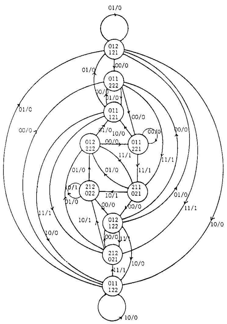
Figure 15. The state transition diagram of a flnite state decode r of M
distance, are not shown here because the main purpose in this linear example is to give an idea about generating the finite state decoder.
Table 1 The next-state and the output table of the decoder M.
| Present | Next | — State | Out | put | |||||
|---|---|---|---|---|---|---|---|---|---|
| Time | State | IN = 00 | IN = 01 | IN = 10 | IN = 11 | 00 | 01 | 10 | 11 |
| 0 | 011 | 011 221 | 011 221 | 011 121 | 211 021 | 0 | 0 | 0 | 1 |
| 1 | 011 121 | 011 222 | 012 121 | 011 122 | 212 021 | 0 | 0 | 0 | 1 |
| 2 | 211 021 | 012 122 | 012 222 | 212 022 | 012 122 | 0 | 0 | 1 | 0 |
| 3 | 011 222 | 011 221 | 012 121 | 011 121 | 212 021 | 0 | 0 | 0 | 1 |
| 4 | 012 121 | 011 222 | 012 121 | 011 122 | 212 021 | 0 | 0 | 0 | 1 |
| 5 | 011 122 | 011 222 | 012 121 | 011 122 | 212 021 | 0 | 0 | 0 | 1 |
| 6 | 212 021 | 012 122 | 012 222 | 212 022 | 012 122 | 0 | 0 | 1 | 0 |
| 7 | 012 122 | 011 222 | 012 121 | 011 122 | 212 021 | 0 | 0 | 0 | 1 |
| 8 | 012 222 | 011 221 | 011 121 | 011 121 | 211 021 | 0 | 0 | 0 | 1 |
| 9 | 212 022 | 012 122 | 012 222 | 212 022 | 012 122 | 0 | 0 | 1 | 0 |
EXAMPLE 2
Figure 16 shows an example of a finite state encoder with three states. The number of decoder states with truncated path length 2 is 79. There are too many to be shown here. The closed path enumeration and identification is computed for \(\alpha = 6\). Table 2 shows the \(F_1\) paths, the \(B_1\) paths and the corresponding closed paths of length 6 in terms of the encoder state sequence.
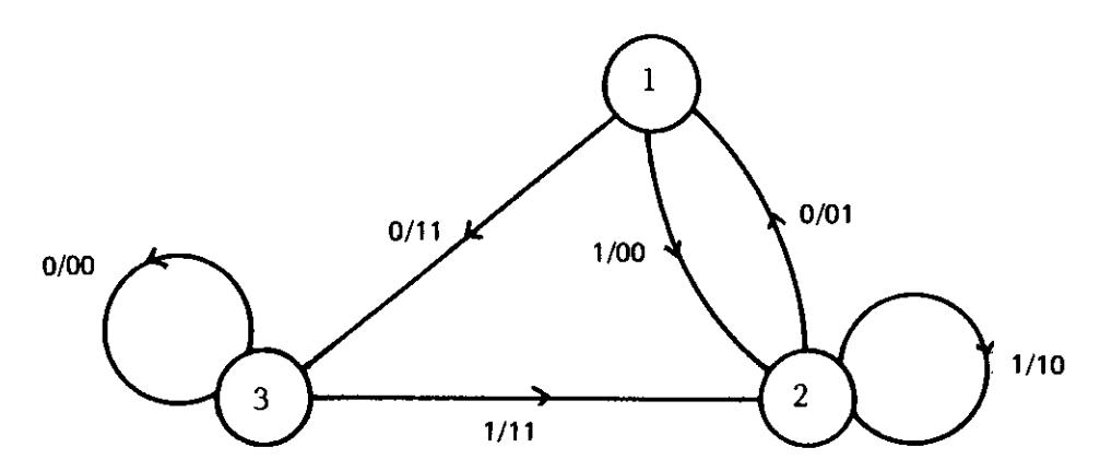
Figurc 16 A finite state encoder /ltv with three states
Table 2 Ttre F1 and the Bl paths and their corresponding closed paths of length 6
| Lengdr | Ft Paths | B I Paths | Cloced Parhs | No |
|---|---|---|---|---|
| o | 13333 | 121 | 1333321 | I |
| '13332 | 221 | 1333221 | ||
| 13321 | 321 | 182121 | ||
| 13322 | 1332221 | 4 | ||
| 13213 | 1321321 | |||
| 13212 | 1321221 | o | ||
| 13221 | 13221?1 | 1 | ||
| 13222 | 1322221 | I | ||
| 12133 | 1213321 | 9 | ||
| 12132 | 12'13221 | 1 0 | ||
| 12121 | 1212121 | 1 l | ||
| 12122 | 1212221 | |||
| 12213 | 1221321 | I J | ||
| 12212 | 1221221 | 1 4 | ||
| 12221 | 1222121 | l 5 | ||
| 12222 | 1222221 | 1 6 |
Table 3 shows the distances among the closed paths of length 6 that diverge and remerge with state l. These distances arc paesented in an n x n matrix form where n is the corresponding closed path; the entry(k,j) is the distance between closed path i and closed path l.
Table 3 The Hamming distances between closed paths of length 6 that diverge from and remerge with state 1
| Cd. Pth. No. | DISTANCE | |||||||||||||||
|---|---|---|---|---|---|---|---|---|---|---|---|---|---|---|---|---|
| 1 | 2 | 3 | 4 | 5 | 6 | 7 | 8 | 9 | 10 | 11 | 12 | 13 | 14 | 15 | 16 | |
| 1 | 0 | 3 | 5 | 4 | 5 | 4 | 6 | 5 | 5 | 8 | 6 | 5 | 6 | 5 | 7 | 6 |
| 2 | 3 | 0 | 4 | 3 | 4 | 5 | 5 | 4 | 8 | 5 | 5 | 4 | 5 | 6 | 6 | 5 |
| 3 | 5 | 4 | 0 | 3 | 6 | 5 | 3 | 6 | 6 | 5 | 5 | 8 | 7 | 6 | 4 | 7 |
| 4 | 4 | 3 | 3 | 0 | 5 | 4 | 6 | 3 | 5 | 4 | 8 | 5 | 6 | 5 | 7 | 4 |
| 5 | 5 | 4 | 6 | 5 | 0 | 3 | 5 | 4 | 6 | 5 | 7 | 6 | 3 | 6 | 8 | 7 |
| 6 | 4 | 5 | 5 | 4 | 3 | 0 | 4 | 3 | 5 | 6 | 6 | 5 | 6 | 3 | 7 | 6 |
| 7 | 6 | 5 | 3 | 6 | 5 | 4 | 0 | 3 | 7 | 6 | 4 | 7 | 8 | 7 | 3 | 6 |
| 8 | 5 | 4 | 6 | 3 | 4 | 3 | 3 | 0 | 6 | 5 | 7 | 4 | 7 | 6 | 6 | 3 |
| 9 | 5 | 8 | 6 | 5 | 6 | 5 | 7 | 6 | 0 | 3 | 5 | 4 | 5 | 4 | 6 | 5 |
| 10 | .8 | 5 | 5 | 4 | 5 | 6 | 6 | 5 | 3 | 0 | 4 | 3 | 4 | 5 | 5 | 4 |
| 11 | 6 | 5 | 5 | 8 | 7 | 6 | 4 | 7 | 5 | 4 | 0 | 3 | 6 | 5 | 3 | 6 |
| 12 | 5 | 4 | 8 | 5 | 6 | 5 | 7 | 4 | 4 | 3 | 3 | 0 | 5 | 4 | 6 | 3 |
| 13 | 6 | 5 | 7 | 6 | 3 | 6 | 8 | 7 | 5 | 4 | 6 | 5 | 0 | 3 | 5 | 4 |
| 14 | 5 | 6 | 6 | 5 | 6 | 3 | 7 | 6 | 4 | 5 | 5 | 4 | 3 | 0 | 4 | 3 |
| 15 | 7 | 6 | 4 | 7 | 8 | 7 | 3 | 6 | 6 | 5 | 3 | 6 | 5 | 4 | 0 | 3 |
| 16 | 6 | 5 | 7 | 4 | 7 | 6 | 6 | 3 | 5 | 4 | 6 | 3 | 4 | 3 | 3 | 0 |
The results of the simulation study are shown in Table 4; it shows the number of bit errors for a particular channel crossover probability and truncated length \(\alpha\) given \(10^4\) uses of the channel.
Table 4 Number of bit errors for a particular crossover probability P and truncated length \(\alpha\) given \(10^4\) uses of the channel
| P | 1 | ||||
|---|---|---|---|---|---|
| · | α = 2 | α = 3 | α = 6 | α = 9 | _ |
| 1. 0x10-2 | 0 | 1 | 1 | 1 | |
| 2. 0x10-2 | 3 | 2 | 2 | 2 | |
| 4. 0x10-2 | 29 | 29 | 22 | 22 | |
| 6. 0x10-2 | 79 | 75 | 56 | 54 | |
| 8. 0x10-2 | 117 | 104 | 98 | 101 | |
| 1. 0x10-1 | 209 | 229 | 187 | 185 | |
| 2. 0x10-1 | 831 | 835 | 754 | 747 |
9 CONCLUSIONS
This paper studied a non-linear class of finite state digital channel coding with the aim of finding some properties of the code which improve the performance. In this case, the performance is measured by the minimum free distance since it is easier to evaluate than the probability of error criterion, and for small channel crossover probability it is a very good indicator of system performance. The analysis has indicated that the structures of the finite state machines are important to performance. In particular, the pairs of closed paths that diverge from and remerge with the same state and how we identify and improve them, in order to find a bigger minimum free distance, are very important; in addition, the catastrophic property has also been investigated, based on the machine structure. Thus, a new approach has been initiated which emphasizes on the structure imposed by modelling our encoder-decoder as a finite state machine; consequently it is not limited to only linear codes. This is in stark contrast to most existing methods of analysis which consider only the class of linear codes.
The general problem itself remains unsolved and there are many aspects of it that may be investigated. Even for the binary case much remains to be done. Although we adopted a truncated version of the Viterbi algorithm for the decoder, we assumed that the system performance could be approximated by the ideal Viterbi algorithm. The analysis of the loss in performance caused by the truncation strategy remains untouched. Consequently, there is a room to improve our bound on bit error probability; a random coding approach could also be used to deal with the error probability measure. Another assumption in our present analysis is that of perfect synchronization. Finding a pair of finite state encoder-decoder that always synchronize is another problem. We mentioned and proved some Markov chain properties, yet we did not exploit these powerful properties. These properties, along with renewal theory, may be useful for the synchronization analysis. The use of a bidirectional search to identify the critical closed paths seems to be helpful. Of course, by the very nature of our algorithm, we can not use this search algorithm if the number of the encoder states is too large. This is a classical problem that remains unresolved when one deals with a graph. In addition, we have not considered the case when the metrics are real numbers. This problem seems much more difficult than the loss of performance due to truncation and code synchronization. We do not know how to deal with this general problem. We leave this as an open problem for further investigations.
ACKNOWLEDGMENTS
The author wishes to express his special gratitude to his thesis advisor, Prof. N.T. Gaarder, whose constant personal guidance and extraordinary patient encouragement in both academic and other matters made all this possible.
Thanks are also due to the members of the thesis committee, Professors Norrnan Abramson and Edward J. Weldoir, Jr., for their criticism, all of which were helpful and constructive.
These studies werc completed while on study leave from the Bandung Institute of Technology and I am grateful to the Institute for this opportunity. Thanks is also due to the East-West Center for its generous financial support.
Finally, I have the geat good fortune to have my Ina as a wife, who assumed the diffrcult role as a wife of a Braduate student on study leave with model grace and undeFtanding. And what we both owe our parents is immeasurable.
R.EFERENCES
- I Elias, P., Coding for Noisy Channels, IRE Conv. Rec., Part 4, pp. 37 -41 , 1955.
- 2 Viterbi, A. J., Error Bounds for Convolutional Codes and an Asymptotically Optimum Decoding Algorithm, IEEE Truts. Theory, vol.IT-13, no. 2, pp. 26O-269, April I 967.
- 3 . . . . . . ., Convolutional Codes and Their Performance in Communications Systems, IEEE Tro* on Commun. Technl., uol. COM-19, no. 5, October 197 | .
- 4 Fomey, G. D., Jr., The Viterbi Algorithm, Proc. IEEE, vol. 61, no. 3, pp. 268-278, Match 1973.
- 5 . . . . . . ., Convolutional Codes I: Algebraic Structur€,IE t Trots. Inform. Theory, vol.IT.. 16, no. 6, pp.72O-738, November 1970.
- 6 . . . . .. ., Convolutional Codes II: Maximum Likelihood Decoding, Inform. and Control, vol. 25, no. 3,pp.222-266, July 1974.
- 7 Larsen, K. J., Short Convolutional Codes with Maximum Free Distance for Rate | 12, ll3, ar;'d, I 14,IEEE Trans. Inform. Theory, vol.IT- 19, no. 3, pp. 37 l-372, May 1973.
- 8 Paaske, E., Short Binary Convolutional Codes with Maximal Free Distance for Rate 213 and 314,IEEE Tron. Inform. Theory, vol. IT-20, no. 5, pp. 683-689, September 1974.
- 9 Johanneson. R. and E. Paaske, Further Results on Binary Convolutional Codes with an Optimum Distance Profile, IEEE Trans. Infonn. Theory, vol.lT-24, no. 2, pp. 264-268, March 1978.
- l0 Costello, D. J., Jr., Free Distance Bounds for Convolutional Codes, IEEE Trans. Inform. Theory, vol.IT-20, no.3,May 1974.
- I I Bahl, L. R., et. al, An Efficient Algorithm for Computing Free Dstance, IEEE Trans. Inform. Theory, vol. IT-18, no. 3, pp. 437 -439, May 1972.
- 12 Lanen, K. J., Comments on 'An Efficient Algorithm for Computing Free Distance', IEEE Trans. Inform. Theory, vol IT-19, no. 4, pp. 577-579, July 1973 .
- l3 Gaarder, N. T. and D. Slepian, On Optimal Finite State Digital Transmission Systems, IEEE Trans. Inform. Theory, vol. IT-28, no. 2, pp. 167 -186, March 1982.
- l4 Wiseman,J. A., A construction of Nonlinear Codes Which Betten of Equals Known Results for Certain Parameten, Inform, od Control, no. 48, pp.7O-79,1981.
- 15 Un, S. and D. J. Costello, Jr., Enor Control Coding: Fundamentals @td Applications. New Jersey: Prentice Hall, 1983.
- l6 Petenon,W. W. and E. J. Weldon, h., Enor Correcting Codes. CambridgB: The MIT Press, 1972.
- 17 Viterbi, A. J. and J. K. Ornura, Principles of Dgital Communication ord Codrhg. New York: McGraw-Hil, 1979.
- l8 Wozencraft, J. M. and I. M. Jacobs, Principles of Communication Engineenng New York: John lViley and Sons, 1965.
- 19 Kohavi,Z., Switching and Finite Automata Theory. New York: McGraw-Hill, 1970.
- 20 Booth,T. L., Sequential Machines and Automata Theory. New York: Wiley, 1967.
- 2l Deo, N., Graph Teory with Applications to Engineeiing and Computer Sciezce. New Jersey: Prentice Hall, 1974.
- 22 Maurer,H- H., Dota Structures and Progamming Techniques. New Jersey: Prentice Hall, 1977.
- 23 Ellis,M. R., A Structurcd Approach to Fortrun 77 Programming. London: Addison-Wesley, 1982.
APPENDIX A
With the notation of section 2 we want to show that \((S_n, R_n)\) is a first order Markov Chain for both the noiseless channel and the additive channel: \(C_n = D_n + N_n\) where + denotes a mod. \(N_C\) addition and the \((N_n)\) are a sequence of independent, identically distributed, random variables.
Proof:
a. Noiseless channel case:
\[\begin{aligned} & Pr[S_n = s_n \& R_n = r_n \mid (S_i, R_i) = (s_i, r_i), i < n - 1] \\ &= Pr[\sigma(X_{n-1}, s_{n-1}) = s_n, \rho(D_{n-1}, r_{n-1}) = r_n \mid (S_i, R_i) = (s_i, r_i), i \le n - 1] \\ &= Pr[\sigma(X_{n-1}, s_{n-1}) = s_n, \rho(\delta(X_{n-1}, s_{n-1}), r_{n-1}) = r_n \mid (S_i, R_i) = (s_i, r_i), i \le n - 1] \\ &= Pr[\sigma(X_{n-1}, s_{n-1}) = s_n, \rho(\delta(X_{n-1}, s_{n-1}), r_{n-1}) = r_n] \\ &= s_n \cdot \delta(x_{n-1}, s_{n-1}) = s_n \cdot \rho(\delta(X_{n-1}, s_{n-1}), r_{n-1}) = r_n] \end{aligned}\]
Hence:
\[Pr[S_n = s_n \& R_n = r_n | S_i = s_i, R_i = r_i, i \le n - 1]\]
= \(Pr[S_n = s_n \& R_n = r_n | S_{n-1} = s_{n-1}, R_{n-1} = r_{n-1}]\)
which completes the proof.
b. Additive channel:
\(C_n = D_n + N_n\) where + denotes a mod. \(N_C\) addition and the \(N_n\) are independent, identically distributed random variables;
\[Pr[S_n = S_n \& R_n = r_n \mid (S_i, R_i) = (S_i, r_i), i \le n - 1]\]
By using our finite state decoder model one can easily get:
\[= Pr \left[ \sigma \left( X_{n-1}, s_{n-1} \right) = s_n, \rho \left( C_{n-1}, r_{n-1} \right) = r_n + (s_i, r_i) = (s_i, m_i), i \le n-1 \right]\] \[= Pr \left[ \sigma \left( X_{n-1}, s_{n-1} \right) = s_n, \rho \left( \delta \left( X_{n-1}, s_{n-1} \right) + N_{n-1}, r_{n-1} \right) = r_n \right]\] \[\left( S_i, R_i \right) = (s_i, r_i), i \le n-1 \right]\] \[= Pr \left[ \sigma \left( X_{n-1}, s_{n-1} \right) = s_n, \rho \left( \delta \left( X_{n-1}, s_{n-1} \right) + N_{n-1}, r_{n-1} \right) = r_n \right]\] since \(S_i\) and \(R_i\) are functions of only \(X_1, \ldots, X_{i-1}\) and \(X_1, \ldots, X_{i-1}\). Hence:
= \(Pr[S_n = s_n \& R_n = r_{n+1}S_{n-1} = s_{n-1}, R_{n-1} = r_{n-1}]\) which completes the proof.
APPENDIX B
With the notation of section 2 we want to show that \((D_n, S_n, Y_n, R_n)\) is a first order Markov Chain for both a noiseless channel: \(C_n = D_n\), and an additive channel: \(C_n = D_n + N_n\) where + denotes a mod. \(N_C\) addition and the \((N_n)\) are independent identically distributed random variables.
Proof:
a. For the noiseless channel: \(C_n = D_n\),
\[\begin{aligned} & Pr\left[D_{n} = d_{n}, S_{n} = s_{n}, Y_{n} = y_{n} \ R_{n} = r_{n} \right] \left(D_{i}, S_{i}, Y_{i}, R_{i}\right) = \left(d_{i}, s_{i}, y_{i}, r_{i}\right), i \leq n - 1 \,] \\ & = Pr\left[D_{n} = d_{n}, \ S_{n} = s_{n}, \ Y_{n} = y_{n}, \ R_{n} = r_{n} \ | D_{n-1} = d_{n-1}, \ Y_{n-1} = y_{n-1}, \\ \left(D_{j}, \ Y_{j}\right) = \left(d_{j}, \ y_{j}\right), j \leq n - 2, \ \left(S_{i}, \ R_{i}\right) = \left(s_{i}, \ r_{i}\right), i \leq n - 1 \,] \end{aligned}\]
By using the finite state model one finds:
\[\text{[rumus tidak dapat ditampilkan dengan baik — lihat PDF asli]}\]
Hence:
\[\begin{aligned} & Pr[D_n = d_n, S_n = s_n, Y_n = y_n, R_n = r_n | D_i = d_i, S_i = s_i, Y_i = y_i, R_i = r_i, i \leq n-1] \\ & = Pr[D_n = d_n, S_n = s_n, Y_n = y_n, R_n = r_n | D_{n-1} = d_{n-1}, S_{n-1} = s_{n-1}, Y_{n-1} = y_{n-1}, R_{n-1} = r_{n-1}] \\ & Y_{n-1} = y_{n-1}, R_{n-1} = r_{n-1}] \\ & \text{which completes the proof.} \end{aligned}\]
b. For additive channel:
\(C_n = D_n + N_n\) where + denotes a mod. \(N_C\) addition and the \(N_n\) are independent identically distributed random variables,
\[\begin{aligned} & Pr[D_{n} = d_{n}, S_{n} = s_{n}, Y_{n} = y_{n}, R_{n} = r_{n} | (D_{i}, S_{i}, Y_{i}, R_{i}) = (d_{i}, s_{i}, y_{i}, r_{i}), i < n - 1] \\ & = Pr[D_{n} = d_{n}, S_{n} = s_{n}, Y_{n} = y_{n}, R_{n} = r_{n} | D_{n-1} = d_{n-1}, Y_{n-1} = y_{n-1}, \\ & D_{j} = d_{j}, Y_{j} = y_{j}, j \le n - 2, S_{i} = s_{i}, R_{i} = r_{i}, i \le n - 1] \end{aligned}\]
By using the finite state model one finds:
= \[Pr[\delta(X_n, \sigma(X_{n-1}, s_{n-1})) = d_n, \sigma(X_{n-1}, s_{n-1}) = s_n,\]
\[\begin{array}{l} \eta \; (\; \delta \; (X_{\rm n}, \sigma (X_{\rm n-1}, s_{\rm n-1})) + N_{\rm n}, \rho (d_{\rm n-1}, r_{\rm n-1})) = y_{\rm n}, \\ \rho (d_{\rm n-1} + N_{\rm n-1}, r_{\rm n-1}) = r_{\rm n} \; | \; D_{\rm n-1} = d_{\rm n-1}, \; Y_{\rm n-1} = y_{\rm n-1} \; ] \; , \\ {\rm since} \; X_{\rm n} \; {\rm and} \; X_{\rm n-1} \; {\rm are} \; {\rm independent} \; {\rm of} \; X_{\rm k} \; {\rm and} \; N_{\rm k} \; {\rm for} \; k < n-2 \; {\rm and} \; {\rm also} \; \\ {\rm independent} \; {\rm of} \; S_{\rm m} \; {\rm and} \; R_{\rm m} \; {\rm for} \; {\rm all} \; m. \end{array}\]
Hence:
\[Pr[D_n = d_n, S_n = s_n, Y_n = y_n, R_n = r_n \mid D_{n-1} = d_{n-1}, S_{n-1} = s_{n-1}, Y_{n-1} = y_{n-1}, R_{n-1} = r_{n-1}]\] which completes the proof.