1 Introduction

Integrable Ha.uriltonian systems, by the Liouville.Arnol'd lntegrability Theorem [1, 11], live in pha^se spaces that are fibrations of invariant tori. Open pieces of the phase space form bundles of Lagrangean tori, where these bundles are not always trivial. An example in two degrees of freedom is given by the spherical pendulum [14, 11], where the nontriviality can be measured by monodromy. [n general nontriviality of such an integrable bundle means the non-existence of global action angle coordinates. Moreover this nontriviality (in particular nontrivial monodromy) turns out to be of great interest in the study of semiclassical versions of such systems [12, 13, 21, 30]. Presently our point of view is perturbative: how persistent is this global bundle geometry under small perturbations of the system? On the one hand these perturbations can be restricted to the world of integrable systems, on the other hand, our main question is what can be said in the near-integrable case.

Here we drop the restriction to two-degrees-of-freedom and resort to the classical Kolmogorov-Arnol'd-Moser Theory for the persistence of Lagrangean invariant tori in nearly-integrable systems. For a general description of this theory see [1, 2, 3, 4]. Sinces resonances are problematic, we have to restrict to quasi-periodic tori with Diophantine frequency vectors. The union of these tori is nowhere dense, but has positive measure, compare [22]. The formulation of present interest is in terms of structural stability [23], for the occasion called quasi-periodic stability. Indeed, following Broer et al. [8, 7], the KAM-Theorem provides a smooth conjugation between the integrable and the near integrable tori. Here the smoothness in the action direction, where the domain of definition due to the resonances has no interior points, has to be understood in the sense of Whitney, see Pöschel [24]. One problem we have to overcome is that this KAM-Theorem is only 'local' in the action directions, suitable for local trivialisations of the bundle. This implies that the global bundle geometry is not carried over directly.

The present paper contains a globalization of these 'local' results to a global kam-Theorem, where the conjugation is glued together from the local ones. Here we use a Partition of Unity construction [16, 26] and also the natural affine structure of the integrable invariant tori [1]. Compare with similar constructions for creating Riemannian metrics or connections, as these occur in Differential Geometry [26]. The main result, as obtained by Broer, Cushman and Fassò [5] is that this construction works, yielding a global diffeomorphism between the integrable and near-integrable torus bundle. If the integrable bundle happens to be nontrivial, so is the near-integrable bundle.

The present paper describes the results in [5], taking the spherical pendulum as a leading example. In the remainder of this section we include a treatment of this example as far as relevant to us. Next, in Section 2 we present a brief treatment of the standard, 'local' KAM-Theory as suited to our purposes. In Section 3 we formulate and prove our main result: the global KAM-Theorem. Finally in Section 5 we draw some conclusions, also briefly revisiting the spherical pendulum.

1.1 Motivation: The spherical pendulum

We describe the dynamics of the spherical pendulum, compare [2, 11, 14, 25]. The spherical pendulum, as suited to our purposes, is a unit mass particle, the motion of which is restricted to the unit sphere \(\mathbb{S}^2 \subseteq \mathbb{R}^3\), where gravity with unit acceleration points vertically downward. The configuration space is the 2-sphere \(\mathbb{S}^2 = \{q \in \mathbb{R}^3 \mid \langle q, q \rangle = 1\}\) and the phase space its cotangent bundle \(T^*\mathbb{S}^2 \cong \{(q,p) \in \mathbb{R}^6 \mid \langle q,q \rangle = 1 \text{ and } \langle q,p \rangle = 0\}\). Here \(q = (q_1,q_2,q_3)\) and \(p = (p_1,p_2,p_3)\), while \(\langle .,. \rangle\) denotes the standard inner product.

The spherical pendulum is a classical integrable system. The rotational symmetry by Noethers Theorem [1] gives rise to a second integral of motion, next to the energy \(E(q,p)=\frac{1}{2}\langle p,p\rangle+q_3\) this is the angular momentum \(I(q,p)=q_1p_2-q_2p_1\), with respect to the vertical axis. The energy-momentum map

\[\mathcal{EM}: T^*\mathbb{S}^2 \to \mathbb{R}^2, (q,p) \mapsto (I,E) = \left(q_1p_2 - q_2p_1, \frac{1}{2}\langle p,p \rangle + q_3\right)\]

has an invariant Lagrangean fibration, where most of the fibers are diffeomorphic to the 2-torus. To be more precise, the image \(\widetilde{B}\) of \(\mathcal{EM}\) is the

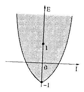
Figure 1: Range of the energy-momentum map of the spherical pendulum.

closed part of the plane lying in between the two curves meeting at a corner, see Figure 1. The set of singular values of \(\mathcal{EM}\) consists of the two boundary curves and the points \((I, E) = (0, \pm 1)\). The latter correspond to the equilibria \((q, p) = (0, 0, \pm 1, 0, 0, 0)\). The boundary curves correspond to the horizontal periodic motions of the pendulum as discovered by Christiaan Huygens. The set B of regular \(\mathcal{EM}\)-values therefore consists of the interior of B minus the point (I, E) = (0, 1), corresponding to the unstable equilibrium point (0, 0, 1, 0, 0, 0), which is a saddle with double eigenvalues \(\pm 1\). The point (I, E) = (0, 1) turns out to be the centre of the nontrivial monodromy.

The corresponding fiber \(\mathcal{EM}^{-1}(1,0)\) is a once pinched 2-torus. See Duistermaat [14] and Cushman-Bates [11]. Note that the fiber \(\mathcal{EM}^{-1}(1,0)\) exactly consists of the coinciding stable and unstable manifolds of the saddle point.

Passing to spherical coordinates

\[q_1 = \sin \phi \cos \theta\], \(q_2 = \sin \phi \sin \theta\) and \(q_3 = \cos \theta\), energy and momentum get the form

\[I = \sin^2 \phi \cdot \dot{\theta}\] \[E = \frac{1}{2} \sin^2 \phi \cdot (\dot{\theta})^2 + \frac{1}{2} (\dot{\phi})^2 + \cos \phi\] \[= \frac{1}{2} (\dot{\phi})^2 + V_I(\phi)\] where

\[V_I(\phi) = \frac{I^2}{2\sin^2\phi} + \cos\phi\] is the effective potential. This is the classical way to exploit the rotational symmetry, or equivalently, that \(\phi\) is a cyclic variable [1]. Thus, for \(I \neq 0\) fixed, we reduce to a standard one degree of freedom system on the phase space \((0,\pi)\times\mathbb{R}=\{\phi,\dot{\phi}\}\) with Hamiltonian function \(E=\frac{1}{2}(\dot{\phi})^2+V_I(\phi)\). It is easy to see that the reduced energy levels are circles of the form \(C_{I,E}=\{(\phi,\dot{\phi})\in(0,\pi)\times\mathbb{R}\mid E=\frac{1}{2}(\dot{\phi})^2+V_I(\phi)\}\). Note that the canonical 1-form is given by \(\sin^2\phi\cdot\dot{\theta}\cdot d\theta+\dot{\phi}\,d\phi\). Integration along \(C_{I,E}\) then leads to the following classical formulæ for the actions:

\[a_1(I, E) = 2\pi I\]
\(a_2(I, E) = 2 \int_{\phi_-}^{\phi_+} \sqrt{2(E - \cos \phi) - \frac{I^2}{\sin^2 \phi}} d\phi\)

where \(\phi_{\pm}\) are defined by \(2(E - \cos \phi_{\pm}) - (I^2/\sin^2 \phi_{\pm}) = 0\).

Next consider the basis \((T_1(I, E), T_2(I, E))\) of the period lattice given by \(T_1(I, E) = (2\pi, 0)\) and \(T_2(I, E) = (T_{2,1}(I, E), T_{2,2}(I, E))\), where

\[T_{2,1}(I,E) = -2I \int_{\phi_{-}}^{\phi_{+}} \frac{1}{\sqrt{2(E - \cos\phi) - \frac{I^{2}}{\sin^{2}\phi}}} \frac{d\phi}{\sin^{2}\phi} = -2 \int_{\phi_{-}}^{\phi_{+}} \frac{\dot{\theta}}{\dot{\phi}} d\phi\] \[T_{2,2}(I,E) = 2 \int_{\phi_{-}}^{\phi_{+}} \frac{1}{\sqrt{2(E - \cos\phi) - \frac{I^{2}}{\sin^{2}\phi}}} d\phi = 2 \int_{\phi_{-}}^{\phi_{+}} \frac{1}{\dot{\phi}} d\phi.\]

Proposition 1 [14] The period functions \(T_1\) and \(T_{2,2}\) are single-valued, while \(T_{2,1}\) is multi-valued. The branching point is \((a_1, a_2) = (0, 0)\), or equivalently (I, E) = (0, 1) and the monodromy matrix is given by

\[\begin{pmatrix} 1 & -1 \\ 0 & 1 \end{pmatrix} \in Sl(2, \mathbb{R}). \tag{1}\]

Taking the appropriate quotients of the period functions yields frequencies \(\omega_1(a_1, a_2)\) and \(\omega_2(a_1, a_2)\). The frequency function \(\omega_1\) is single-valued, whereas \(\omega_2\) is multi-valued.

Already by the Liouville-Arnol'd Integrability Theorem [1] it follows that locally—with respect to the actions \((a_1, a_2)\)—we have canonical action-angle variables \((a_1, a_2, \alpha_1, \alpha_2)\) in which the motions of the spherical pendulum are given by

\[\dot{a}_1 = 0 \dot{a}_2 = 0 \dot{\alpha}_1 = \omega_1(a_1, a_2) \dot{\alpha}_2 = \omega_2(a_1, a_2).\] (2)

The actions \(a_1\) and \(a_2\) have replaced the integrals I and E as constants of motion. Fixing \(a_1\) and \(a_2\) gives an invariant 2-torus, parametrized by \(\alpha_1\) and \(\alpha_2\), on which the motion is parallel with frequency vector \(\omega(a_1, a_2)\). The nontriviality of the 2-torus bundle means that the angle variables in (2) can not be extended over the whole domain: global action angle variables do not exist.

Remark The monodromy matrix (1) indicates a certain shift in the periodor frequency lattice when moving in a circle around the branching point, see Figure 1. Such a lattice also occurs in the spectrum of the Schrödinger operator in a semiclassical version of the spherical pendulum, where a similar shift is observed. Compare with [12, 30].

1.2 Perturbative point of view; setting of the problem

The spherical pendulum is an example of an integrable system in the sense of Liouville-Arnol'd [1], where the torus bundle is nontrivial. It is natural to ask whether this property is persistent for perturbations of the system. Let us first consider the case where the perturbations do not lead us out of the class of integrable systems. The following result largely characterizes the integrable cases in two-degrees-of-freedom.

Theorem 1 [19, 29] Given a four dimensional symplectic manifold M fibered by level sets of an energy momentum map \(\mathcal{EM}: M \to \mathbb{R}^2\). Assume that

• 1. EM has only one critical value;
• 2. Each fiber of EM is compact and connected:
• 3. The singular fiber has k singular points, all real or complex saddle points (also named focus-focus points).

Then the singular fiber is a pinched torus and the Liouville-Arnold 2-torus bundle is nontrivial, where in a suitable basis the monodromy matrix takes the form

\[\left(\begin{array}{cc} 1 & -k \\ 0 & 1 \end{array}\right) \in Sl(2, \mathbb{R}).\]

It directly follows that the monodromy of the 2-torus bundle related to the spherical pendulum is persistent for small integrable (say rotationally symmetric) Hamiltonian perturbations of the system.

A next question is whether this geometry also is persistent for non-integrable Hamiltonian perturbations. Think of applying a non-symmetric magetic field to the spherical pendulum. This question and related issues form the motivation for the present paper.

First, we drop the restriction to two-degree-of-freedom systems and turn to the general Hamiltonian setting with n degrees of freedom. Second, we aim to use Kolmogorov-Arnol'd-Moser Theory [24, 8, 7] in its quasi-periodic stability format, comparing near-integrable systems to their integrable approximation. In [5] it is shown that this approach is successful: below we shall explain these results further. As we shall see it will be possible to construct a global Whitney smooth diffeomorphism between the integrable and near-integrable n-torus bundle with an Whitney extension that respects the geometry. We note that this approach is independent of the particular geometry of the integrable approximation.

2 'Local' KAM Theory

In this section we review the standard, 'local' Kolmogorov-Arnol'd-Moser Theory [24, 8, 7] for nearly-integrable Hamiltonian systems in n degrees of freedom, also compare [10, 18]. As said before, this theory deals with the persistence of invariant Lagrangean n-tori, that are quasi-periodic.

2.1 Conditions on the integrable approximation

The phase space we consider is \(\mathbb{T}^n \times A\), where \(A \subset \mathbb{R}^n\) is a bounded, open and connected subset. The adjective 'local' to KAM-Theory refers to the fact that the theory deals with local trivializations of the whole n-torus bundle.

Let \((\alpha, a) = (\alpha_1, \ldots, \alpha_n, a_1, \ldots, a_n)\) be a set of action angle coordinates on \(\mathbb{T}^n \times A\), where the symplectic form is given by \(\sum_{j=1}^n da_j \wedge d\alpha_j\). Compare [1, 11].

Let \(h: \mathbb{T}^n \times A \to \mathbb{R}\) be a smooth Hamilton function, integrable, in the sense of not depending on the angles \(\alpha\). This leads to a Hamiltonian vector field \(X_h\)

\[X_h(\alpha, a) = \sum_{j=1}^n \omega_j(a) \frac{\partial}{\partial \alpha_j}\], with \(\omega_j = \frac{\partial h}{\partial a_j}\), \(j = 1, 2, \dots, n\).

Note that \(X_h\) has the 2n-dimensional system form

\[\dot{a} = 0 \dot{\alpha} = \omega(a),\] (3)

compare with the spherical pendulum example (2). We say that the system is nondegenerate whenever the frequency map \(\omega: A \to \mathbb{R}^n\) is a diffeomorphism.

We now need to consider the non-resonance condition on the frequency vectors. Given a fixed constant \(\tau > n-1\) and a 'parameter' \(\gamma > 0\), we define

\[D_{\gamma}(\mathbb{R}^n) = \{ \omega \in \mathbb{R}^n \mid |\langle \omega, k \rangle| \ge \gamma |k|^{-\tau}, \forall k \in \mathbb{Z}^n \setminus \{0\} \}\]

We say that the frequency vector \(\omega\) is Diophantine if for some \(\tau > n-1\) and \(\gamma > 0\) we have \(\omega \in D_{\gamma}(\mathbb{R}^n)\). Observe that Diophantine frequency vectors surely are non-resonant. The set \(D_{\gamma}(\mathbb{R}^n)\) is nowhere dense set and of positive measure, which tends to full measure as \(\gamma \downarrow 0\). Compare [24, 8, 7]. For general background on such sets compare [22].

2.2 Formulation of the 'local' KAM Theoren

We need to specify some domains in the frequency and in the action space. For \(\Gamma = \omega(A) \subseteq \mathbb{R}^n\) let

\[D_{\gamma}(\Gamma_{\gamma}) = \{ \omega \in \Gamma \mid \operatorname{dist}(\omega, \partial \Gamma) > \gamma \} \cap D_{\gamma}(\mathbb{R}^n)\]

also define \(D_{\gamma}(A_{\gamma}) \subset A\) by \(D_{\gamma}(A_{\gamma}) = \omega^{-1}(D_{\gamma}(\Gamma_{\gamma}))\). It follows that measure \[(A \setminus D_{\gamma}(A_{\gamma})) = O(\gamma)\] as \(\gamma \downarrow 0\).

Next we perturb the integrable Hamiltonian h to \(h+f:\mathbb{T}^n\times A\to\mathbb{R}\), where we assume both h and f real-analytic. Introducing a complexified domain

\[D_{\varrho,\kappa} = (\mathbb{T}^n + \kappa) \times (A + \varrho),\]

\(\varrho < 1\), we assume h + f is holomorphic here. Here we abbreviated

\[A + \varrho = \{ z \in \mathbb{C}^n \mid |z - a| \le \varrho \text{ for some } a \in A \},\] and similarly for \(\mathbb{T}^n + \kappa \subseteq \mathbb{C}/(2\pi\mathbb{Z})^n\).

Theorem 2 [24, 8] Under the above circumstances, assume that the integrable Hamiltonian system defined by h is nondegenerate. Then there exists a constant \(\delta > 0\), independent of A, \(\gamma\) and \(\varrho\) with the following property. For \(|f|_{D_{\varrho,n}} \leq \gamma^2 \delta\) there exists a map \(\Phi : \mathbb{T}^n \times A \to \mathbb{T}^n \times A\) such that

• 1. \(\Phi\) is \(C^{\infty}\) diffeomorphism, analytic in \(\alpha\);
• 2. \(\Phi\) Id is small in the \(C^{\infty}\)-topology;
• 3. Abbreviating \(\widehat{\Phi} = \Phi|_{\mathbb{T}^n \times \mathcal{D}_{\gamma}(A_{\gamma})}\) we have \(\widehat{\Phi}_* X_h = X_{h+f}\).

The star-notation just abbreviates \(\widehat{\Phi}_{\star}X_h(q)=D_p\widehat{\Phi}(X_h(p))\), where \(\widehat{\Phi}(p)=q\), which indeed amounts to smooth conjugation of the corresponding flows. Theorem 2 is the stability formulation of the standard KAM Theorem. In this format the map \(\Phi\) generally is not symplectic. Since \(\Phi\) is near-identity diffeomorphism, it preserves the topology (geometry) of the bundle. For more details see below. Note that outside \(\mathbb{T}^n \times D_{\gamma}(A_{\gamma})\) the diffeomorphism \(\Phi\) generally is no conjugation. The 'parameter' \(\gamma\) in the 'local' KAM Theorem 2, for all practical purposes, should be as small as perturbation allows. In particular, when writing the perturbation as \(h + \varepsilon f\), we take \(\gamma = O(\sqrt{\varepsilon})\). In general \(\gamma\) may depend on system parameters.

For simplicity we formulated Theorem 2 in the world of real analytic systems, endowed with the compact-open topology on holomorphic extensions. We note that this setting can be relaxed to can be relaxed to \(C^k\), endowed with the Whitney \(C^k\)-topology, when k is sufficiently large. For details see [24, 8]. Also see [9].

3 The global KAM Theorem

Here we give the main result of this paper, the global KAM Theorem. We start with a section that introduces all the necessary ingredients.

3.1 Ingredients

We start out from a real analytic symplectic manifold \((\tilde{M}, \sigma)\), with \(\dim \tilde{M} = 2n\). Moreover, there exists a real analytic surjective map \(\tilde{\pi}: \tilde{M} \to \tilde{B}\), where \(\tilde{B}\) is an n-dimensional affine manifold. Assume that the regular leafs of \(\tilde{\pi}\) are Lagrangean n-tori. Let \(B \subset \tilde{B}\) be the set of regular values of \(\tilde{\pi}\), then we assume that \(M = \tilde{\pi}^{-1}(B)\) is connected. Let \(\pi: M \to B\) be both the restriction and corestriction of \(\tilde{\pi}\).

By the Liouville-Arnol'd Integrability Theorem [1, 11], for all \(b \in B\) we obtain a neighbourhood \(U^b \subset B\) and a map \(\varphi : \pi^{-1}(U^b) \to \mathbb{T}^n \times A^b\) of the form

\[m \mapsto (\alpha^b(m), a^b(m)),\] which is an action angle chart, meaning that the action functions \(a^b = (a_1^b, a_2^b, \ldots, a_n^b)\) are constant on the fibers of \(\pi\).

Let a real analytic Hamiltonian \(H: \tilde{M} \to \mathbb{R}\) be given, which is integrable in the sense that H is constant on the fibers of \(\tilde{\pi}\). This means that the corresponding Hamiltonian vector field \(X_H\) is tangent to fibers of \(\tilde{\pi}\) so that the push forward vector field \(\varphi^b_*X_H\) has the form \(\varphi^b_*X_H = \sum_{j=1}^n \omega^b_j(a) \, \partial/\partial \alpha_j\). Compare with (2) and (3). As before \(\omega^b: A^b \to \mathbb{R}^n\) is called the frequency map. For this construction compare [27, 28].

3.2 Formulation of the global KAM Theorem

We say that H is a nondegenerate integral of \(\tilde{\pi}\), if for the collection \((\pi^{-1}(U^b), \varphi^b)_{b \in B}\) each frequency map \(\omega^b: A^b \to \mathbb{R}^n\) is diffeomorphic onto its image. Using the affine structure on \(\tilde{B}\) the second derivative \(D^2H\) can be defined intrinsically and this nondegeneracy condition then can equivalently be expressed by requiring \(D^2H\) to have maximal rank everywhere.

Now consider any open, relatively compact subset \(B'\subset B\) and define \(M'=\pi^{-1}(B').\) Our main result is

Theorem 3 [5] Let \((M, \sigma)\), \(\pi: M \to B\) and \(H: M \to \mathbb{R}\) be as above and let \(F: M \to \mathbb{R}\) be real analytic. Then, if the restriction \(F|_{\pi^{-1}(B')}\) is sufficiently small in compact-open topology, there exists a subset \(C \subset B'\) and a map \(\Phi: M' \to M'\) such that

• 1. C is a nowhere dense set with measure (C) large;
• 2. \(\Phi\) is a \(C^{\infty}\) diffeomorphism, near the identity in the \(C^{\infty}\) topology;
• 3. For \(\widehat{\Phi} = \Phi|_{\pi^{-1}(C)}\) we have \(\widehat{\Phi}_* X_H = X_{H+F}\).

Remark It is of interest to reconsider Theorem 3 in the case where the perturbation H+F is integrable as well. In that case the proof below runs completely similar, where the 'local' KAM-Theorem 2 is replaced by the Inverse Function Theorem, compare with [8], §3. Therefore there is no need of Diophantine non-resonance conditions and the map \(\Phi\) coincides with its restriction \(\widehat{\Phi}\). So \(\Phi\) is a real analytic diffeomorphism defined on the whole torus bundle, which moreover is an isomorphism of torus bundles and which is a conjugation everywhere. We conclude that if H is globally nondegenerate and H+F is integrable, then the dynamics of H and H+F are analytically conjugate by a global torus bundle isomorphism.

4 Proof of the global KAM Theorem

The rest of the paper is devoted to proving Theorem 3, following Broer, Cushman and Fassò [5].

4.1 Preliminaries

First of all, for each chart domain \((V^b, \varphi^b)_{b \in B}\), we take \(\gamma^b > 0\) small enough such that

\[V_{\gamma^b}^b = (\varphi^b)^{-1}(\mathbb{T}^n \times A_{\gamma^b})\] is a nonempty set of positive measure. For our relatively compact subset \(B' \subset B\) we find a finite sub-covering \((V_{\gamma^j}^j)_{j=1}^N\) of M'.

Localisation For each \(1 \leq j \leq N\) the chart map \(\varphi^j : V^j \to \mathbb{T}^n \times A^j\) leads to a local perturbation problem for \(h^j + f^j\) by defining \(h^j = H \circ (\varphi^j)^{-1}\) and \(f^j = F \circ (\varphi^j)^{-1}\). For each \(1 \leq j \leq N\) application of the 'local' KAM Theorem 2 gives a smooth map \(\Phi^j : \mathbb{T}^n \times A^j \to \mathbb{T}^n \times A^j\), such that restricted to \(D_{\gamma^j}(A^j_{\gamma^j})\) we have

\[\widehat{\Phi^j}_* X_{h_i} = X_{h_i + f_i}.\]

Therefore, each Diophantine invariant torus T of \(X_H\), by a composition

\[(\varphi^j)^{-1} \circ \Phi^j \circ \varphi^j\] is conjugate to an invariant torus T' of \(X_{H+F}\).

The nowhere dense set C Recall the format of the chart map being \(\varphi^j: V^j \to \mathbb{T}^n \times A^j, m \mapsto (\alpha^j(m), a^j(m))\). The set \(C \subset B'\) is obtained by pulling back \(D_{\gamma^j}(A^j_{\gamma^j})\) along \(a^j: V^j \to A^j\). On the finitely many overlaps \(V^i_{\gamma^j} \cap V^j_{\gamma^j}\) we just take intersections.

Matching How do the local conjugacies \((\varphi^j)^{-1} \circ \Phi^j \circ \varphi^j\) match? By nondegeneracy of H the correspondence between the Diophantine integrable tori T and their near-integrable counterparts T' is uniquely determined. Moreover, on any overlap \(V^i_{\gamma^i} \cap V^j_{\gamma^j}\) the actions \(a^i\) and \(a^j\) match under the transition maps \(\varphi^i \circ (\varphi^j)^{-1}\).

However, note that the angles do not necessarily match. Indeed, generally one has \(\alpha^j = S_{i,j}\alpha^i + c_{i,j}\), for \(S_{i,j} \in Sl(n,\mathbb{Z})\) and \(c_{i,j} \in \mathbb{T}^n\), compare [11, 15]. In the case of nontrivial monodromy the transition maps \(\varphi^i \circ (\varphi^j)^{-1}\) are not all close to Id whence we do not always have \(S_{i,j} = \mathrm{Id}\).

4.2 Staying near the identity-map

To overcome the problem of the non-matching angles, for j = 1, 2, ..., N, we consider the near-identity map

\[\Psi^j := (\varphi^j)^{-1} \circ (\Phi^j)^{-1} \circ \varphi^j : T' \to T.\]

The Liouville-Arnol'd Integrability Theorem [1, 11] provides a natural affine structure of the integrable torus T, determined by the transitive \(\mathbb{R}^n\)-action of \(G: \mathbb{R}^n \times T \to T\), as

\[G:((t_1,\ldots,t_n),m)\mapsto (g_1^{t_1}\circ\cdots\circ g_n^{t_n}(m)),\] where \(g_{\ell}^{t}\) is the flow of the Hamiltonian vector field \(X_{a_{\ell}^{j}}\), associated to action \(a_{\ell}^{j}\), for \(\ell = 1, \ldots, n, j = 1, \ldots, N\).

Lemma 1 For sufficiently small F, on any overlap \(T \subset V_{\gamma^i}^i \cap V_{\gamma^j}^j\)

• 1. The transition maps \(\Psi^i \circ (\Psi^j)^{-1}\) are close to \(\operatorname{Id}\) in the \(C^\infty\)-topology
• 2. \(\Psi^i|_{T'}\) and \(\Psi^j|_{T'}\) differ only by a translation

Proof Directly from the equicontinuity conditions on the size of \(\{f^j\}_{j=1}^N\).

Glueing the \(\Psi^j\) A final essential ingredient for glueing the \(\Psi^j\) is

Lemma 2 Subordinate to the covering \((V_{\gamma^b}^b)_{b\in B}\) of M there exists a Partition of Unity \((V_{\gamma^{\lambda}}^{\lambda}, \xi^{\lambda})_{\lambda\in\Lambda}\) with

\[\xi^{\lambda}: M \to \mathbb{R}, \text{ of class } C^{\infty}\]

such that

• 1. (^ is constant on the fibers of r;
• 2. supp(()) e Vl^ * o compact set;
• 3. {^ takes uolues in [0, 1];
• 4. D^rr€^ = I os o (locally) fnite sum.

Proof Take a standard Partition of Unity construction [16, 26] with to the covering (Ult)aen of B and pull back along zr. respect tr

Conclusion of the proof We now conclude this section by a proof of Theorem 3. We define a conjugacy O, as required, by setting

\[\Phi^{-1} := \sum_{j=1}^N \xi^j \Psi^j.\]

This formula has to be interpreted fiber wise as follows. In each integrable ? the maps ilrt and lVj only differ by a translation. The finite convex combination therefore is globally well-defined on the nowhere dense set n-'(C). That the map is near-identity in the C--topology follows by Leibniz' rule. This proves the global KAM Theorem 3. !

Remark The affine structure of T also is determined by its quasi-periodic flow. The KAM conjugations transport this to ?'. Moreover, the global conjugation Q is an isomorphism of bundles, which preserves this affine structure.

5 Conclusions

In this section we first come back to the spherical pendulum example and then draw some further conclusions from our general approach, pointing at a few open problems.

5.1 The spherical pendulum revisited

In any application of Theorem 3 ii is important to verify global nondegeneracy of the Hamiltonian. In the case of the spherical pendulum this fact was established by Horozov [17]. This means that one can apply Theorem 3 to any open, relatively compact subset B' c B. Here the smallness condition on the perturbation depends on B'. Compare Figure 1. However, near the boundary lines corresponding to Huygens's horizontal periodic solutions and near both equilibria, we can send \(\gamma \downarrow 0\), so obtaining Lebesque density points of quasi-periodicity. Compare [8, 7] also compare the problem of small twist as treated in [24].

Suitable Whitney extension of the map \(\Phi\) allows the definition of monodromy in non-integrable, small perturbations of the spherical pendulum. Compare with Rink [25], who establishes this same fact near general focus-focus singularities in two degrees of freedom.

5.2 General remarks

Observe that the present approach works in arbitrary many degrees of freedom and is independent of the integrable geometry one starts with. Suitable Whitney extension of the map \(\Phi\) allows to conclude that near-integrable n-torus bundles are diffeomorphic to their integrable approximations, implying that the geometries are identical. Thus all kinds of obstructions against triviality, like monodromy, Chern classes, etc., can also be defined for the near-integrable case. For a topological discussion of the corresponding n-torus bundles, see Duistermaat [14]. As we saw, the main tool is that near-identity torus-automorphisms are translations [11, 15].

A direct generalization of this approach is possible to the setting of Broer et al. [8, 7], where a general unfolding theory of quasi-periodic tori is developed, based on [20, 24]. Within the world of Hamiltonian systems this leads to applications at the level of lower dimensional tori. However, this approach also works for, e.g., dissipative, volume preserving, or reversible systems. Also compare [6].

An open problem is how to define such obstructions by a more direct approach that tries to take appropriate sections in appropriate bundles. Indeed, remaining with the monodromy example for a while, we see that \(Sl(n, \mathbb{Z})\)-elements play role when jumping over larger gaps in 'Cantor' set C. Thus more monodromy seems to be 'collected along the way' ...

Acknowledgements

The author thanks Richard Cushman, Francesco Fassò, Bob Rink, Mikhail Sevryuk, Carles Simó and Floris Takens for helpful discussion.