

Introduction
In this survey paper we will sketch some recent developments on compound sums and their statistical applications in finance. First we briefly discusstatistical estinratiolr of the total claim size I total error anlount in insurance/accountancy applications. Second. we propose and investigate a simple estimator of the probability of ruin in the Poisson risk model. for the special case where the claim sizes are assumed to be exponentiaJly distributed.
Let S, : L?=, Zr, n : 1,2,. . ., denote the partial sums of nonnegative independent and identically distributed (i.i.d.) random variables (r.v.'s) 21,22,. . ., with common distribution function (d.f.) fl. In insurance applications .9, can be interpreted ns the arrival time of claims. That is, St : Zr is the arrival time of the first claim. Sz = Zt * 22 the arrival time of the second claim, etc. Define the renewal counting process {A/(r),, 2 0} by
\[N(t) = \max\{n : S_n \le t\} \tag{1.1}\]
i.e. rV(l) is the number of claim anivals in [0,t]. If H(a): I - exp(-Br), e ) 0, that is the claim inter-arrival times Zt, Zz,. . . are exponentia.lly distributed with parameter B, then {1/(r),, > 0} is a Poisson process with intensity (rate) 0, 0 > 0.
This means that the process \(\{N(t), t \geq 0\}\) has independent increments: the number of claims that occur in disjoint time intervals are independent, while the number of claims in any interval of length t is Poisson distributed with mean \(\beta t\): for all \(s, t \geq 0\)
\[P(N(t+s) - N(s) = n) = e^{-\beta t} \frac{(\beta t)^n}{n!} , \quad n = 0, 1, \dots\] (1.2)
Note that (1.2) implies that the Poisson process \(\{N(t), t \geq 0\}\) has stationary increments and its mean value is equal to \(EN(t) = \beta t\).
A compound Poisson process \(\{S_{N(t)}, t \geq 0\}\) with rate \(\beta\) is given by
\[S_{N(t)} = \sum_{i=1}^{N(t)} X_i , \quad t \ge 0\] (1.3)
where \(\{N(t), t \geq 0\}\) is a Poisson process with rate \(\beta\), and \(\{X_i, i \geq 1\}\) is a family of i.i.d. r.v.'s with common d.f. F, also independent of \(\{N(t), t \geq 0\}\). For any fixed t, the random variable \(S_{N(t)}\) is called a compound Poisson sum or a random Poisson sum.
It is well known that
\[\frac{S_N - \nu \mu}{\sqrt{\nu \mu_2}} \xrightarrow{d} N(0, 1) , \text{ as } \nu \to \infty\] (1.4)
where \(S_N = S_{N(t)}\), \(\nu = EN(t) = \beta t\), the expected number of claims in [0,t], and \(\mu = \int x \ dF(x)\), whereas \(\mu_2 = \int x^2 \ dF(x)\) is assumed to be finite. Here N(0,1) denotes a standard normal r.v. Note that in insurance applications \(ES_{N(t)} = \nu \mu\) denotes the total claim size in a portfolio in [0,t]. We refer to Gnedenko & Korolev [4] for an excellent account of the general theory for compound sums.
As a first statistical application we want to establish a confidence interval for \(ES_N = \nu \mu\), the total claim size. Let us assume that claim sizes \(X_1, \ldots, X_N\) are observed. An approximate normal based confidence interval for \(ES_N\), with confidence level \(1 - \alpha\), is given by
\[\left(S_N - u_{\alpha/2} \left(\sum_{i=1}^N X_i^2\right)^{1/2}, S_N + u_{\alpha/2} \left(\sum_{i=1}^N X_i^2\right)^{1/2}\right)\] (1.5)
where \(u_{\alpha/2} = \Phi^{-1}(1 - \alpha/2)\). Here \(\Phi\) denotes the standard normal d.f. This is a simple consequence of (1.4), a central limit theorem for Poisson compound sums. However, the normal approximation for compound sums usually performs very badly, because typically the distribution of the \(X_i\), that is the claim size distribution F in insurance applications, is highly skewed to the right. One may look for better methods for approximating the distribution of a compound sum, e.g. the bootstrap or empirical Edgeworth/saddle point approximations. To obtain a more accurate confidence interval for the total claim size \(ES_N\) than the normal-based interval (1.5) one has to consider a Studentized Poisson compound sum
\[\frac{S_N - \nu \mu}{(\sum_{i=1}^N X_i^2)^{1/2}} \tag{1.6}\]
instead of \((S_N - \nu \mu)/\sqrt{\nu \mu_2}\) (see (1.4)), and establish an Edgeworth expansion for the d.f. of (1.6):
\[P\left(\frac{S_N - \nu\mu}{(\sum_{i=1}^N X_i^2)^{1/2}} \le x\right) = \Phi(x) + \frac{1}{6\sqrt{\nu}} \frac{\mu_3}{\mu_2^{3/2}} (2x^2 + 1)\phi(x) + o(1/\sqrt{\nu}) , \qquad (1.7)\] as \(\nu \to \infty\). Here \(\mu_3 = EX_1^3\), and \(\phi\) denotes the standard normal density. In addition to the standard normal limiting distribution \(\Phi\) for a Studentized compound sum, we correct for skewness by means of a term of order \(1/\sqrt{\nu}\) in the Edgeworth expansion. With the aid of the expansion (1.7) one can obtain an improved Edgeworth-based confidence interval for \(ES_N\). For statistical applications one has to replace the skewness coefficient \(\nu^{-1/2}\mu_3/\mu_2^{3/2}\) in (1.7) by its empirical counterpart \(\sum_{i=1}^N X_i^3/(\sum_{i=1}^N X_i^2)^{3/2}\). Another possibility would be to employ the bootstrap and/or use empirical saddlepoint approximations. This is work in progress (see [7] and [10]).
Our second application arises in statistical auditing (see [6]), where one attempts to check the validity of financial statements of a firm or a government agency. Compound sums like \(S_N\) naturally show up in this context as well. In these accountancy applications \(S_N\) denotes the "total error amount" in a random sample of size n drawn without replacement from an audit population of "book amounts"; the \(X_i\), \(1 \le i \le N\), are the nonzero errors observed by the accountant in n recorded "book values"; N is the random number of book values in the sample of size n with error. In typical applications errors are rare, that is the probability that the errors are non zero is close to zero, and the Poisson approximation for N works well. Clearly \(\frac{T}{n}S_N\) is an unbiased estimator of the total error amount in an audit population of size T. In [6] a new upper confidence limit for the total error amount in an audit population - or for \(\frac{T}{n}ES_N = \frac{T}{n}\nu\mu\) - is obtained. The method involves an empirical Cornish-Fisher expansion in the first stage; in the second stage we employ the bootstrap to calibrate the coverage probability of the resulting interval estimate.
Next we will briefly describe the Poisson risk model, which is a simple model for the risk in an insurance portfolio based on the compound Poisson process \(\{S_{N(t)}, t \geq 0\}\) and discuss (see section 2) the statistical estimation of ruin probabilities in this model. The risk can be described as risk = initial capital + income - outflow, and the risk reserve process up to time t can be modelled as
\[R(u,t) = u + ct - S_{N(t)}, \quad t \ge 0\] (1.8)
where \(u \ge 0\) is the initial capital and c > 0 is the premium rate; note that for any fixed t, \(S_{N(t)} = \sum_{i=1}^{N(t)} X_i\) is a Poisson compound sum. By ruin we mean the event \(\{S_{N(t)} > u + ct\}\): the income u + ct at time t of the insurance company is smaller than the total claim \(S_{N(t)}\) to be paid to the customers.
Note that we assume that premium income is linear in time with rate c > 0 and we do not take into account neither the interest income for the accumulated reserve nor the expenses, taxes and dividends etc. \(S_{N(t)} = \sum_{i=1}^{N(t)} X_i\) is the total claim size (or aggregate claim amount) up to time t. If N(t) = 0, define \(S_{N(t)} = 0\). This model is also known as the classical Cramer-Lundberg model for insurance risk.
Figure 1 shows a realization of a risk reserve process (1.8): we see that both the third claim which occurs at time \(\tau = Z_1 + Z_2 + Z_3\) and the fourth claim at time \(\tau' = \tau + Z_4\) yield a value of the risk reserve process below zero. Hence, \(\tau\) denotes the first time that ruin occurs; \(\tau\) is a defective r.v. and \(P(\tau < \infty)\) denotes the probability that ruin will happen at least once; the event \(\{\tau = \infty\}\) corresponds to the case that R(u,t) is nonnegative for any \(t \geq 0\): no zero crossing of the risk reserve process will occur in \((0,\infty)\).
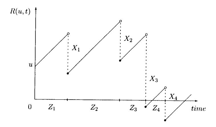
Figure 1 One realization of the risk reserve process R(u,t)
It is clear that, for any fixed u, the process R(u,t) increases linearly with slope c until a claim occurs, at which point the process has a downward jump, since the value of \(S_{N(t)}\) increases at these points.
\(\mathbf{T}\)
G
Definition For any \(u \ge 0\) and \(0 < T < \infty\), the probability of ruin in "finite time horizon" [0,T] is given by
\[\Psi(u,T) = P(R(u,t) < 0 \text{ for some } t < T).\]
The probability of ruin in "infinite time horizon" is defined as \(\Psi(u, \infty) = \lim_{T\to\infty} \Psi(u, T)\); or in other words:
\[\Psi(u) = \Psi(u, \infty) = P(R(u, t) < 0 \text{ for some } t \ge 0) , \quad u \ge 0 , \tag{1.9}\] that is, \(\Psi(u) = P(\tau < \infty)\). In section 2 we will focus on the statistical estimation of the probability of ruin \(\Psi(u)\) for the special case that the claim sizes \(X_i\), \(1 \le i \le N\), are i.i.d. with exponential distribution with mean \(\lambda\), \(\lambda > 0\). That is, F is \(\exp(1/\lambda)\). In this very special case the probability of ruin \(\Psi(u)\) has a simple form: for any \(u \ge 0\),
\[\Psi(u) = \begin{cases} \frac{\lambda \beta}{c} \exp\left(-u(\frac{1}{\lambda} - \frac{\beta}{c})\right) & ; \text{ if } \lambda < c/\beta \\ 1 & ; \text{ otherwise } . \end{cases}\] (1.10)
For practical applications in insurance, statistical estimation of \(\Psi(u,T)\), for T=10 years, say, is perhaps more interesting; in the present paper we focus on a simpler problem of estimating \(\Psi(u)\). Note that \(\Psi(u) \geq \Psi(u,T)\), for any T>0; typically the error we make in replacing \(\Psi(u,T)\) by \(\Psi(u)\) is quite small. In this connection we want to mention that as early as in 1955 H. Cramér showed that if \(u\to\infty\), \(T\to\infty\) and \(u^2/T\to0\), then \(\Psi(u)-\Psi(u,T)\) gets exponentially small (see Jensen (1995) [12] page 300, for details).
The condition \(\lambda < c/\beta\) is known as the net profit condition, and also as the positive safety loading \(\rho\) condition where \(1+\rho=c/\beta\lambda\). To verify (1.10) we recall the well-known general formula for the probability of ruin under the net profit condition \(\lambda < c/\beta\) and u > 0:
\[\Psi(u) = (1 - \frac{\lambda \beta}{c}) \sum_{r=1}^{\infty} (\frac{\lambda \beta}{c})^r (1 - G^{(r)}(u)) , \qquad (1.11)\] where \(G(x) = \frac{1}{\lambda} \int_0^x (1 - F(y)) dy\) and \(G^{(r)}\) denotes the r-fold convolution of G with itself; \(\Psi(u) = 1\) if \(\lambda \ge c/\beta\). We refer to Asmussen [1] page 63, or Rolski et al. [14] page 164, as well as Embrechts et al. [3] page 29. In the important special case that \(F(x) = P(X \le x) = 1 - e^{-x/\lambda}\), G reduces to
\[G(u) = \frac{1}{\lambda} \int_0^u (1 - (1 - e^{-y/\lambda})) dy = \int_0^x \frac{1}{\lambda} e^{-y/\lambda} dy = 1 - e^{-u/\lambda}.\]
This means that not only F but also G is \(exp(1/\lambda)\), and consequently \(G^{(r)}\) is \(Gamma(r, 1/\lambda)\). By a standard argument, the formula for \(\Psi(u)\) in (1.11) can now be simplified as follows:
\[\Psi(u) = (1 - \frac{\lambda \beta}{c}) \sum_{r=1}^{\infty} (\frac{\lambda \beta}{c})^r \left( 1 - \int_0^u \frac{\frac{1}{\lambda} e^{-y/\lambda} (y/\lambda)^{r-1}}{(r-1)!} dy \right) = (1 - \frac{\lambda \beta}{c}) \sum_{r=1}^{\infty} (\frac{\lambda \beta}{c})^r \int_u^{\infty} \frac{\frac{1}{\lambda} e^{-y/\lambda} (y/\lambda)^{r-1}}{(r-1)!} dy = (1 - \frac{\lambda \beta}{c}) \int_u^{\infty} \left( \sum_{r=1}^{\infty} (\frac{\lambda \beta}{c})^r \frac{\frac{1}{\lambda} e^{-y/\lambda} (y/\lambda)^{r-1}}{(r-1)!} \right) dy = (1 - \frac{\lambda \beta}{c}) \int_u^{\infty} \left( \frac{\beta}{c} e^{-y/\lambda} \sum_{r=1}^{\infty} (\frac{y\beta}{c})^{r-1} \frac{1}{(r-1)!} \right) dy = (1 - \frac{\lambda \beta}{c}) \int_u^{\infty} \frac{\beta}{c} e^{-y/\lambda} e^{y\beta/c} dy = \lambda (1/\lambda - \beta/c) \frac{\beta}{c} (1/\lambda - \beta/c)^{-1} e^{-u(1/\lambda - \beta/c)} = \frac{\lambda \beta}{c} \exp(-u(1/\lambda - \beta/c)),\] which is precisely (1.10).
2 Statistical estimation of the probability of ruin
We consider the Poisson risk model for the special case that the claim size d.f. .P is exp(1/)), with /r dF(r) = ), so that the infinite time probability of ruin has the simple form given in (1.10). Let rc denotes the expected inter-claim arrival tirne E21. Clearly n: l/F.
Let us suppose that a single realization (past data) of the compound Poisson process with rate I f n, S 1,1111 = I-tq) Xi, is observecl in a bourrded window (interval) [4/, which expands in time. That is, weobserve the inter-arrival tirnes {Z;} and the clainr sizes {X;} occurring in 17. Let u: EN(W): /lwl: lWlln denotes the expected number of claim arrivals in W; lWl denotes the size or Lebesque r)ea.sure of l/ and y can be viewed as the expected sample size of our data set. Ftom a single realization Slo(,), I e W, one can compute
\[\widehat{\lambda}_{\bar{N}} = \frac{1}{\bar{N}} \sum_{i=1}^{\bar{N}} X_i \quad \text{and} \quad \widehat{\kappa}_{\bar{N}} = \frac{1}{\bar{N}} \sum_{i=1}^{N} Z_i , \qquad (2.1)\] where N is the number of observed claims, provided at least one claim is observed in I4z. If N : N(W) : 0, no claims have occurred in W - our data set is empty and statisticalestimation (of V(u)) is clearly impossible. Note that N : N I N > 1, i.e. \(\bar{N}\) is a zero truncated Poisson r.v. Clearly \(EN^{-1} = \infty\), while it can be checked that \(E\bar{N}^{-1} \sim \nu^{-1}\), or more accurately (see [8])
\[E\bar{N}^{-1} = \nu^{-1} + \nu^{-2} + 2\nu^{-3} + 6\nu^{-4} + o(\nu^{-4})\], as \(\nu \to \infty\). (2.2)
Asymptotic expansions like (2.2) enable us to obtain asymptotic approximations for the central moments of the empirical mean of claim sizes \(\hat{\lambda}_{\bar{N}}\) and inter-claim arrival times \(\hat{\kappa}_{\bar{N}}\) (c.f. (2.1)). In practice the exact times of the claim arrivals may not be known to the insurance company, that is, the \(Z_i\)'s were not observed, only the total number of claims \(\tilde{N}(W)\) in W is observed. In this situation \(\hat{\kappa}_{\bar{N}}\) cannot be computed; instead one may estimate \(\kappa\) by \(|W|/\bar{N}(W)\). Note that (2.2) directly yields that \(E(|W|/\bar{N}(W)) = \kappa \nu (\nu^{-1} + \mathcal{O}(\nu^{-2})) = \kappa + \mathcal{O}(\nu^{-1})\), as \(\nu \to \infty\).
We estimate the probability of ruin \(\Psi(u)\) with its plug-in estimate, which is obtained by simply replacing the unknown parameters \(\lambda\) and \(\kappa\) by their empirical counterparts \(\widehat{\lambda}_{\bar{N}}\) and \(\widehat{\kappa}_{\bar{N}}\):
\[\widehat{\Psi}_{\bar{N}}(u) = \begin{cases} \frac{\widehat{\lambda}_{\bar{N}}}{c \ \widehat{\kappa}_{N}} \exp\left(-u\left(\frac{1}{\widehat{\lambda}_{\bar{N}}} - \frac{1}{c \ \widehat{\kappa}_{N}}\right)\right) & ; \text{ if } \widehat{\lambda}_{\bar{N}} < c \ \widehat{\kappa}_{\bar{N}} \\ 1 & ; \text{ otherwise } . \end{cases}\] \[(2.3)\]
Throughout this paper we will assume that both the initial capital u and the premium rate c are known to the insurance company. One can check that the estimates \(\widehat{\lambda}_{\bar{N}}\) and \(\widehat{\kappa}_{\bar{N}}\) have the (weak) consistency property: as \(\nu \to \infty\), then \(\widehat{\lambda}_{\bar{N}} \stackrel{p}{\longrightarrow} \lambda\) and \(\widehat{\kappa}_{\bar{N}} \stackrel{p}{\longrightarrow} \kappa\). Asymptotic normality of \(\widehat{\Psi}_{\bar{N}}(u)\) can also be established, whenever \(\lambda < c\kappa\).
Theorem For any fixed u, as \(v \to \infty\),
\[\sqrt{\nu} \left( \widehat{\Psi}_{\bar{N}}(u) - \Psi(u) \right) \xrightarrow{d} N(0, \tau^2)\] where \(\tau^2 = \tau^2(u) = [\Psi(u)]^2 [(1 + u/\lambda)^2 + (1 + u/(c\kappa))^2]\), provided that \(\lambda < c\kappa\). Moreover, if \(\lambda > c\kappa\), then as \(\nu \to \infty\),
\[\widehat{\Psi}_{\bar{N}}(u) \xrightarrow{a.s.} 1\].
In fact, if \(\lambda > c\kappa\), the much stronger assertion \(P(\widehat{\Psi}_{\bar{N}}(u) = 1) = 1 - P(\widehat{\lambda}_{\bar{N}} \le c\widehat{\kappa}_{\bar{N}}) = 1 - \mathcal{O}(e^{-d\nu})\), as \(\nu \to \infty\), for some constant d > 0, also holds true (c.f Lemma). In the border case \(\lambda = c\kappa\) a non-normal weak limit for \(\sqrt{\nu}(\widehat{\Psi}_{\bar{N}}(u) - 1)\) appears. We refer to [9] for details.
Sketch of proof. We first consider the case that \(\lambda < c\kappa\). Write
\[\begin{array}{rcl} A_{\bar{N}} & = & \sqrt{\nu} (\widehat{\Psi}_{\bar{N}}(u) - \Psi(u)) I(\widehat{\lambda}_{\bar{N}} < c \ \widehat{\kappa}_{\bar{N}}) \\ B_{\bar{N}} & = & \sqrt{\nu} (\widehat{\Psi}_{\bar{N}}(u) - \Psi(u)) I(\widehat{\lambda}_{\bar{N}} \ge c \ \widehat{\kappa}_{\bar{N}}) \ , \end{array}\] then \(\sqrt{\nu}(\widehat{\Psi}_{\bar{N}}(u) - \Psi(u)) = A_{\bar{N}} + B_{\bar{N}}\). For any fixed \(u \geq 0\) one can prove that \(A_{\bar{N}} \stackrel{d}{\to} N(0, \tau^2)\) and \(B_{\bar{N}} \stackrel{p}{\to} 0\), as \(\nu \to \infty\). Then Slutsky's theorem yields the desired result. The main term \(A_{\bar{N}}\) can be analyzed by a Taylor expansion \((\Psi(u))\) is differentiable in \(\lambda\) and \(\kappa\)) and the remainder term \(B_{\bar{N}}\) can be shown to be negligible by means of the lemma below. We refer to [9] for a complete proof.
Finally we consider the case that \(\lambda > c\kappa\). The claim is that, if \(\lambda > c\kappa\), then \(\widehat{\Psi}_N(u) \xrightarrow{a.s.} 1\), as \(\nu \to \infty\). To check this we note that \(\widehat{\Psi}_{\bar{N}}(u) \xrightarrow{a.s.} 1\) if \(\widehat{\lambda}_{\bar{N}}/c\widehat{\kappa}_{\bar{N}} \xrightarrow{a.s.} \lambda/c\kappa\), because of (2.3). The latter requirement, however, is a simple consequence of the (strong) consistency property of \(\widehat{\lambda}_{\bar{N}}\) and \(\widehat{\kappa}_{\bar{N}}\): as \(\nu \to \infty\), then \(\widehat{\lambda}_{\bar{N}} \xrightarrow{a.s.} \lambda\) and \(\widehat{\kappa}_{\bar{N}} \xrightarrow{a.s.} \kappa\).
In fact, see also [9], one can show that the theorem remains valid if not only \(\nu \to \infty\), but also \(u \to \infty\), provided \(u/\sqrt{\nu} \to 0\). This is of much importance in insurance applications, as typically the initial capital u is large and the probability of ruin will be quite small. If both u and \(\nu\) approach infinity, while \(u/\sqrt{\nu} \to 0\), we obtain
\[\frac{\sqrt{\nu}}{u} \left( \frac{\widehat{\Psi}_{\tilde{N}}(u)}{\Psi(u)} - 1 \right) \stackrel{d}{\longrightarrow} N \left( 0, \frac{1}{\lambda^2} + \frac{1}{(c\kappa)^2} \right) , \qquad (2.4)\]
provided \(\lambda < c\kappa\). If u is fixed, then (2.4) yields the classical order \(\nu^{-1/2}\) for the random deviations \(\widehat{\Psi}_{\bar{N}}(u)/\Psi(u)-1\). On the other hand, if \(u\to\infty\), but \(u=o(\sqrt{\nu})\), then the order of magnitude of the relative error \(\widehat{\Psi}_{\bar{N}}(u)/\Psi(u)-1\) is of a larger order, namely \(u/\sqrt{\nu}\). In view of (2.4), the quantity \(\nu/u^2\) can be seen as the order of magnitude (up to a constant factor determined by the scale (currency) of u) of the "effective sample size" for estimating \(\Psi(u)\), as both \(\nu\) and u get large.
In Figure 2 we see that indeed very large data sets (that is, a very large value of \(\nu\)) seem to be needed before "asymptotic normality" really starts to work. In the left panel, normality clearly fails to hold: the Q-Q plot shows that the distribution of \(\widehat{\Psi}_N(u)\) is highly skewed to the right. In this case \(\nu=10^4\), \(u=10^3\), so that \(u/\sqrt{\nu}=10\). In the other two panels the cases \(\nu=10^6\), \(u=10^3\), respectively \(\nu=10^8\), \(u=10^3\), are displayed, corresponding to \(u/\sqrt{\nu}=1\) and 1/10 respectively. Clearly the distribution of \(\widehat{\Psi}_N(u)\) is much closer to the normal in these two cases. We refer to Hipp [11] for some related work.
To conclude this section we present a simple and useful lemma which shows that in a certain sense our estimator (2.3) for \(\Psi(u)\) behaves as one would hope. The lemma also serves as an important technical tool in our asymptotic analysis; for instance, it is used in the proof of the theorem. However, the lemma is more general in scope, as it will also be useful when investigating estimators for the probability of ruin in the Poisson risk model with general claim size d.f. F, that is, estimators of \(\Psi(u)\) given by (1.11).
hat ed er-
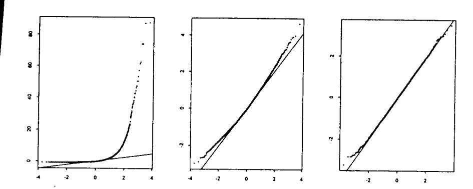
Figure 2: Normal Q-Q plots of \(\widehat{\Psi}_{\bar{N}}(u)\) based on 5000 realizations of (2.3) simulated in \(W = [0, \kappa \nu]\), where \(\nu = 10^4\) (left), \(\nu = 10^6\) (middle), and \(\nu = 10^8\) (right); with \(\kappa = 10\), \(\lambda = 9.5\), c = 1, u = 1000. The true probability of ruin \(\Psi(u) = 0.00492\).
The estimator (2.3) of the probability of ruin \(\Psi(u)\) will take the value 1 if and only if \(\widehat{\lambda}_{\bar{N}} \geq c\widehat{\kappa}_{\bar{N}}\). The following lemma tells us that, if \(\lambda < c\kappa\), this unpleasant event will happen with exponentially small probability as \(\nu\) gets large, provided Bernstein's condition is satisfied. This is confirmed by the simulations for various large values of \(\nu\) reported in Figure 2: none of the 15.000 values of \(\widehat{\Psi}(u)_N\) were found to be equal to 1.
Lemma Suppose that the common distribution F of the i.i.d. claim sizes \(X_i\), \(i = 1, 2, \ldots\) satisfies Bernstein's condition: for \(m = 2, 3, \ldots\) and some positive constants K and R we have
\[E_F \mid X_1 - EX_1 \mid^m \le m! K^{m-2} R^2 / 2\] (2.5)
If \(\lambda < c\kappa\), then there exists a positive constant \(d_1\) (depending on \(\lambda\) and \(\kappa\)) such that
\[P(\widehat{\lambda}_{\tilde{N}} \ge c \ \widehat{\kappa}_{\tilde{N}}) = \mathcal{O}\left(e^{-d_1\nu}\right) \text{ , as } \nu \to \infty \ .\] (2.6)
Similarly, if \(\lambda > c\kappa\), then \(P(\widehat{\lambda}_{\bar{N}} \leq c \ \widehat{\kappa}_{\bar{N}}) = \mathcal{O}(e^{-d_2\nu})\), as \(\nu \to \infty\).
Sketch of proof. The basic probabilistic tool to prove this lemma is a well-known property of the Poisson process: conditionally given that \(\bar{N}=n\), the arrival time \(\sum_{i=1}^n Z_i\) of the nth claim has exactly the same distribution as the distribution of the maximum of a random sample of size n from the uniform d.f. on W=(0,T), where \(T=\kappa\nu\). That is, \(\mathcal{L}(\sum_{i=1}^{\bar{N}} Z_i \mid \bar{N}=n)=\mathcal{L}(T|U_{n:n})\), with \(U_{n:n}\) denotes the maximum of a sample of size n from the Uniform(0,1) distribution. In view of the preceding argument we can write
\[P(\widehat{\lambda}_{\tilde{N}} \ge c \ \widehat{\kappa}_{\tilde{N}}) = \sum_{n=1}^{\infty} P\left(\sum_{i=1}^{n} X_i \ge cTU_{n:n}\right) P(\tilde{N} = n) \ . \tag{2.7}\]
We split the summation in (2.7) in two parts: \(\mathbb{N} = I \cup I^c\), with \(I = \{n \in \mathbb{N} : | n - E\bar{N} | < \epsilon \sqrt{E\bar{N}} \}\) for some fixed \(\epsilon > 0\). Then,
\[P(\hat{\lambda}_{\bar{N}} \ge c \ \hat{\kappa}_{\bar{N}}) \le \sum_{n \in I} P\left(\sum_{i=1}^{n} X_i \ge cTU_{n:n}\right) + \sum_{n \in I^c} P(\bar{N} = n) \ . \tag{2.8}\]
The second term in (2.8) can be bounded as follows:
\[\sum_{n \in I^c} P(\tilde{N} = n) = P\left(\frac{|\tilde{N} - E\tilde{N}|}{\sqrt{E\tilde{N}}} \ge \epsilon\right) \le \frac{2}{1 - e^{-\nu}} \exp\left(\frac{-\epsilon^2}{2 + \epsilon/\sqrt{\nu}}\right). \tag{2.9}\]
The latter inequality is nothing but an exponential bound for zero-truncated Poisson r.v.'s, which can be easily established by slightly modifying the proof of a well-known exponential bound for Poisson r.v.'s (see Reiss [13] page 222).
Taking \(\epsilon = \epsilon(\nu, a) = a\sqrt{\nu}\) for some constant a > 0, it is easy to check from (2.9) that
\[\sum_{n \in I^c} P(\bar{N} = n) = \mathcal{O}\left(e^{-d\nu}\right) , \text{ as } \nu \to \infty.\] (2.10)
with \(d = a^2/(2+a) > 0\). It remains to evaluate the first term on the right hand side of (2.8). To check that this term is also of exponentially small order one can appeal to Bernstein's inequality (c.f. (2.5)). We refer to [9] for complete details.
Note that Bernstein's condition (2.5) is easily checked to be valid for the case that F is \(\exp(1/\lambda)\), \(\lambda > 0\). Bernstein's condition also holds true for many other d.f.'s F, but typically fails for heavy-tailed claim size d.f.'s. An interesting example of a claim size d.f. F for which Bernstein's condition (2.5) fails is the Pareto d.f., \(F(x) = 1 - (1 + x)^{-2}\), for \(x \ge 0\). For this simple heavy-tailed model we have that \(\int x \, dF(x)\) is finite, but \(\int x^2 \, dF(x) = \infty\). A simple calculation based on Theorem 2.1.a of Gut [5] shows that, if \(\lambda < c\kappa\), then in the Pareto model we have that \(P(\widehat{\lambda}_{\bar{N}} \ge c\widehat{\kappa}_{\bar{N}}) \to 0\), as \(\nu \to \infty\), at a fairly slow rate, namely slightly slower than \(\nu^{-1}\). Hence, any estimator of the probability of ruin (1.11), which would involve \(\widehat{\lambda}_{\bar{N}}\) and \(\widehat{\kappa}_{\bar{N}}\) will presumably work less well in such heavy-tailed models, then it does in cases where Bernstein's condition is satisfied. The case that \(\lambda\) and \(\kappa\) are known, but F (and hence G) is unknown and must be estimated from the data, was considered by Croux & Veraverbeke [2].
3 Acknowledgement
The research of the second author wa.s supported by the Royal Netherlands Academy of Arts and Sciences (KNAW).