

1 Introduction
To makc optimal decisions is onc of the most basic desires of a humau being. Whenever the situatioo and the targets admit a tractable mathematical formalization, this desire can. to some extent, be met by tools offered by the optimization theory and algorithms. A very general mathematical setting of an optimization problem is the following:
\[\min_{x \in X} \{ f_0(x) : f_i(x) \le 0, i = 1, \dots, m \}.\] (P)
In this problem, we are given an objective function /s(r) and finitely many functional constraints fi@) S 0,f = 1,...,ffi. The fuuctions /,(r) are realvalued functions of an n-dirrensional design vector r varying iu a given domain X. The goal is to minimize the objective over the feasible set of the problem, i.e., the set which is cut off the domain X by the system of inequalities fi@) < 0,i : 1, ,..,ffi. In general, this is a very hard problem to solve. Tbe situation is much better if all functions /r(r),i :0, 1,...,rn are convex. In that case (P) is callcd a Convex Optimization problem. But even thcn, the problem might be hard to solve.
In this paper we restrict ourselvcs to a special class of coDvex optimization problcm, namcly Conic Optimization (CO) problcms. Conic optirnization addrcsses the problem of minimizing a linear objcctivc function ovcr thc interscction of an a{fine set and a convcx cone. The general form is as follows
\[\min_{x \in \mathbf{R}} \left\{ c^T x : Ax - b \in \mathcal{K} \right\}. \tag{CP}\]
In T] la fic fo: ca oF ap TI ill of aF tr ot T' bc ex ap dc TI in, pr dc A fCi su Bi fo. th SC m de to pc ml a '
TI Sel re' rcl
Thc objcctivc function is cTr, with objcctive vcctor c € Rn. Furthcrmorc, Ar - b rcprcscnts an affinc function from Rt' to R- and K dcnotcs a convex conc in R-. Usually ,4 is given as an rn x n (constraint) matrix, and b e R-. Thc importancc of this class of problcurs is due to two facts: first nrany nonlincar problcms can bc modclled as a conic optimization problcm, and, sccondly, undcr some wcak conditions on the underlying conc K, conic optimization problcms can bc solvcd cfficicntly.
Thc most ca^sy and most wcll known casc occurs whcn thc conc K is thc nonnegativc orthant of Rt', i.c. whcn K : R?:
\[\min_{x \in \mathbf{R}} \left\{ c^T x : Ax - b \in \mathbf{R}_+^m \right\}. \tag{LO}\]
This is nothing clsc as onc of thc standard forrns of thc wcll known Lincar Optimization (LO) problcnr. Thus it bccorncs clcar that LO is a spccial casc of CO. It is wcll known that LO nrodcls covcr numcrous applications. Whcncvcr applicable, LO allows to obtain uscful quantitativc and qualitativc inforrnation on thc problem at hand. Thc spccific analytic structure of an LO problcm givcs risc to a numbcr of gcncral rcsults which providc in many cascs valuablc insight and undcrstanding. At thc sanre timc, this analytic structurc undcrlics somc spccific conrputational tcchniqucs for LO; thcsc techniqucs, which by now arc pcrfcctly well dcvclopcd, allow to solvc routincly quitc large (with tcns/hundreds of thousands of variables and constraints) LO problems. Ncvcrthclcss, thcrc arc many situations in rcality which cannot be covcrcd by LO nrodcls. To handlc thcsc "esscntially nonlinear" cases, thcrc is a strong nccd to extcnd thc basic thcoretical rcsults and computational tcchnioucs known for LO beyond the bounds of LO.
Whcn passing from a generic LO problcm to its nonlinear extcnsions, we should expcct to cncounter some nonlinear componcnts in the problcm. Historically, this was done by putting thc nonlincarity in the functions defining the problcm, as donc above in problem (P). In conic optimization, however, we rcplacc thc conc R! in (LO) by a nonlinear convcx conc K, and hence thc nonlinearity is now captured in thc cone. In the ncxt section wc discuss somc basic propcrtics of rclevant convcx cones and we introduce two spccial cones that play promincnt role in thc contcxt of conic optimization.
In the recent years, a lot of attention has been devoted to conic optimization. The rcason is that the interior-point mcthods that were developed in the two last decades for LO (see, e.g., ll9, 22, 24, 23)), and which revolutionized the field of LO, could be naturally cxtended to obtain polynomial-time mefhods for CO (see, e.g. [18]). This opened the way to a wide spectrum of new applications which cannot be captured by LO, e.g. in control thcory, combinatorial optimization, ctc. For a complete survey both of the theory of CO and its applications, wc refer to the recent book [8].
The aim of thc paper is to introduce thc rcader to thc theory of CO, and to illustratc its use. LO has a beautiful duality theory. Wc will see that much of this thcory can be gcncralized to CO. Wc dcal with onc of the important applications of conic optimization, namely truss topology design (TTD). A truss is a mechanical construction comprising thin elastic bars linkcd to cach other, such a^s an clectric mast, a railroad bridgc, or the Eiffel towcr. The TTD problcnr dcals with how to design an optimal truss, with a givcn wcight, best able to withstand a givcn load. The TTD problcm hers bccn studicd cxtcnsiveiy, both mathematically and algorithrnically .1,2,5,13, 17, 25]. The approach in this paper is mainly bascd on [8]; somc ncw cxarnplcs of truss designs arc given in the course of thc papcr.
The papcr is organizcd as follows. Section 2 introduccs thc theory of CO including the main duality rcsults for CO. Scction 3 is dcvoted to the TTD problem. A nonlincar and a linear model of the singlc load TTD problenr arc derived in Scction 3.1. ln *,his scction wc givc thrce examplcs of truss dcsigns. A fourth cxamplc is uscd to dcrnonstrate the instability of thc dcsign with respcct to additional loads, in Scction 3.1.7. Thc samc cxamplc is uscd in subscqucnt scctions to show how more stablc dcsigns can bc obtaincd.
Bascd on a variational principlc, introduced in Section 3-2.1, wc derivc a modcl for thc TTD problcm that enablcs us to dcal with the multi-load casc, i.e., thc ca^sc whcre we want to dcsign a truss that is able to withstand a finitc sct of diffcrcnt loads in the best possiblc way. The model is a conic optimization modcl, of the semidcfinitc typc. A simple cxamplc of a multi-load design is prcscntcd, and it is shown that the ncw dcsign may be vcry scnsitive to smali occa,$ionaloads. Finally, to make the design less sensitive to such pcrturbations in the load, in Section 3.2.4 we make use of a recently devclopcd modclling tcchnique (sce, e.g., [3, 4, 6, 7, 9, 10, 11, 12, 14, 15, 211) that yiclds a very robust design.
Conic optimization
Thc gcncral form of a conic optimization problem is as given by (CP). In this section wc start with a discussion of thc conditions on thc cone ,C, and wc review the threc most important cones. Then we deal with the main duality results for CO. It will become clear that under some mild conditions the duality
theory for CO closely resembles the well known duality theory for LO.
2.1 More on convex cones
Recall that a subset K of \(\mathbb{R}^m\) is a cone if
\[a \in \mathcal{K}, \lambda \ge 0 \Rightarrow \lambda a \in \mathcal{K},\] (1)
and the cone K is a convex cone if moreover
\[a, a' \in \mathcal{K} \Rightarrow a + a' \in \mathcal{K}.\] (2)
We will impose three more conditions on \(\mathcal{K}\). Recall that CO is a generalization of LO. To obtain duality results for CO similar to those for LO, the cone \(\mathcal{K}\) should inherit three more properties from the cone underlying LO, namely the nonnegative orthant:
\[\mathbf{R}_{+}^{m} = \left\{ x = (x_{1}, \dots, x_{m})^{T} : x_{i} \geq 0, i = 1, \dots, m \right\}.\]
This cone is called the linear cone. The linear cone is not just a convex cone; it is also pointed, it is closed and it has a nonempty interior. These are exactly the three properties we need. We describe these properties now. A convex cone \(\mathcal K\) is called pointed if it does not contain a line. This property can be stated equivalently as
\[a \in \mathcal{K}, -a \in \mathcal{K} \Rightarrow a = 0.\] (3)
A convex cone K is called closed if it is closed under taking limits:
\[a_i \in \mathcal{K} \ (i = 1, 2, \ldots), \ a = \lim_{i \to \infty} a_i \Rightarrow a \in \mathcal{K}.\] (4)
Finally, denoting the interior of a cone K as int K, we will require that
\[int \mathcal{K} \neq \emptyset. \tag{5}\]
This means that there exists a vector (in \(\mathcal{K}\)) such that a ball of positive radius centered at the vector is contained in \(\mathcal{K}\). In conic optimization we only deal with cones \(\mathcal{K}\) that enjoy all of the above properties. So we always assume that \(\mathcal{K}\) is a pointed and closed convex cone with a nonempty interior. Apart from the linear cone, two other relevant examples of such cones are
1. The Lorentz cone
\[\mathbf{L}^{m} = \{ x \in \mathbf{R}^{m} : x_{m} \ge \sqrt{x_{1}^{2} + \ldots + x_{m-1}^{2}} \}.\]
This cone is also called the second-order cone, or the ice-cream cone.
2. The positive semidefinite cone \(\mathbf{S}_{+}^{m}\). This cone "lives" in the space \(\mathbf{S}^{m}\) of \(m \times m\) symmetric matrices (equipped with the Frobenius inner product \(\langle A, B \rangle = Tr(AB) = \sum_{i,j} A_{ij} B_{ij}\)) and consist of all \(m \times m\) matrices A which are positive semidefinite, i.e.,
\[\mathbf{S}_{+}^{m} = \left\{ A \in \mathbf{S}^{m} : x^{T} A x \ge 0, \quad \forall x \in \mathbf{R}^{m} \right\}.\]
We assume that the cone \(\mathcal K\) in (CP) is a direct product of the form
\[\mathcal{K} = \mathcal{K}^1 \times \ldots \times \mathcal{K}^m,\] where each component \(\mathcal{K}^i\) is either a linear, a Lorentz or a semidefinite cone.
2.2 Conic Duality
Before we derive the duality theory for conic optimization, we need to define the dual cone of a convex cone K:
\[\mathcal{K}_{\star} = \left\{ \lambda \in \mathbf{R}^{m} : \lambda^{T} a \ge 0, \, \forall a \in \mathcal{K} \right\}.\] (6)
We recall the following result from [8].
Theorem 2.1 Let \(K \subset \mathbb{R}^m\) is a nonempty cone. Then
- (i) The set K* is a closed convex cone.
- (ii) If K has a nonempty interior (i.e., int \(K \neq \emptyset\)) then \(K_*\) is pointed.
- (iii) If K is a closed convex pointed cone, then int \(K_* \neq \emptyset\).
- (iv) If K is a closed convex cone, then so is \(K_*\), and the cone dual to \(K_*\) is K itself.
Corollary 2.2 If \(K \subset \mathbb{R}^m\) is a closed pointed convex cone with nonempty interior then so is \(K_*\), and vice versa.
One may easily verify that the three cones introduced in Section 2.1 arc self-dual. The dual of a direct product of convex cones is the direct product of their duals, i.e.,
\[\mathcal{K} = \mathcal{K}^1 \times \ldots \times \mathcal{K}^m \quad \Rightarrow \quad \mathcal{K}_* = \mathcal{K}_*^1 \times \ldots \times \mathcal{K}_*^m.\]
As a consequence, any direct product of linear, Lorentz and semidefinite cones is self-dual.
Now we are ready to deal with the problem dual to a conic problem (CP). We start with observing that whenever x is a feasible solution for (CP) then the definition of K- implies )" (,4e - b) > 0, for all ) € K*, and hence c satisfies the scalar inequality
\[\lambda^T A x \ge \lambda^T b, \quad \forall \lambda \in \mathcal{K}_*.\]
It follows that whenever ) € K. satisfies the relation
\[A^T \lambda = c \tag{7}\] then one has
\[c^T x = (A^T \lambda)^T x = \lambda^T A x \ge \lambda^T b = b^T \lambda\] for all r fcasible for (CP). So, if .\ e ,C* satisfies (7), then the quantity bTl is a lowcr bound for the optimal valuc of (CP). The best lower bound obtainablc in this way is the optimal valuc of thc problcm
\[\max_{\lambda \in \mathbf{R}} \left\{ b^T \lambda : A^T \lambda = c, \, \lambda \in \mathcal{K}_* \right\}.\] (CD)
By definition, (CD) is the dual problem of (CP). Using Theorem2.I (iu), onc casily verifies that the duality is symmctric: thc dual problcm is conic and the problem dual to the dual problem is the primal problem.
Indccd, from thc construction of thc dual problcm it immcdiatcly follows that we have the weak duality property: if s is fcasible for (CP) and ) is fcasiblc for (CD), then
\[c^T x - b^T \lambda \ge 0.\]
Thc crucial question is, of course, if we havc cquality of the optimal valucs whcncvcr (CP) and (CD) havc optimal valucs. Diffcrcnt from thc LO casc, howcver, this is in gcneral not the case, unlcss some additional conditions arc satisfied. The following thcorem clarifies thc situation. For its proof wc rcfcr again to [8]. We call the problem (C P) solvablc if it has a (finite) optimal valuc, and this value is attained. Before stating the thcorem it may be worth pointing out that a finite optimal value is not necessar:ily attained. For cxample, thc problem
\[\min_{x} \left\{ x : \left( \begin{array}{cc} x & 1 \\ 1 & y \end{array} \right) \succeq 0 \right\}\]
has optimal value 0, but one may easily verify that this value is not attained. We need one morc definition: if therc exists an rl such that Ar - b e int K then wc say that (CP) is strictly feasible. We have similar, and obvious, dcfinitions for (C D) bcing solvablc and strictly fcasible, rcspcctively.
Theorem 2.3 Let the primal problem (C P) and its dual problem (C D) be as giuen aboue. Then one has
(i) a. If (CP) is below bounded, and strictly feasible, then (CD) is soluable and the rvspectiue optimal ualues are equol.
- b. If (C D) is aboue bounded and strictly feasible, then (C P) is soluable, and the rcspectiae optimol ualues are equal.
- (ii) Suppose that at least one of the two problerns (C P) and (C D) is bounded and strictly feasible. Then a primal-dual feasible pair (r, A) is comprised of optimal solutions to the respectiue problems
- a. if and only if br A : cTs (zero duatity gap).
- b. if and only if Xr[,lx b] : 0 (complementary slackness).
Notc that this rcsult is slightly wcaker than the corresponding result for thc LO case. In the LO case the same thcorem holds by putting cvcry'whcrc "fcasiblc" instcad of "strictly feasiblc". The adjective "strictly" cannot bc omittcd hcrc, howcvcr. For a morc cxtcnsivc discussion and sornc appropriatc countcrexamplcs wc rcfcr to [8].
3 The truss topology design problem
A truss is a mcchanical construction comprising thin clastic bars linkcd to each other, such a^s an electric mast, a railroa<l bridgc, or thc Eiffel towcr. Thc points at which thc bars are linkcd to cach othcr arc callcd thc nodcs of the truss. A truss can bc subjcctcd to an cxtcrnal load a collection of simultancous forces acting at the nodcs, as shown by cxamplc in Figurc 1. Somc nodcs of thc truss arc fixcd nodcs (likc thc nodcs A, B and ,,1' in thc figurc), whcrcas thc rcmaining nodcs are callcd frcc nodes. In somc of thc frec nodcs (nodcs C, C' and.E in thc figurc) an cxtcrnal load acts on thc truss.
Figure 1: A simple planar truss with a load
Under the load. the truss deforms a bit, until the forces in the bars caused by the deforrnation, compensate the external forces. When deformed, the truss stores certain potential enerry; this energy is called the compliance of the truss with respect to the load. The less the compliance, the more rigid the truss is with respect to the load in questton.
Our goal is to design a truss of a given total weight best able to withstand a given load. We call this the TTD problem.
This section is organized as follows. First we derive a linear model for the single load case and give some examples. 6Flom the exarnples it becomes clear that the solution obtained from the linear model can be very instable with respect to occasional small additional loads. This makes it necessary to consider the case of multi-loads. This case cannot be modelled in a linear way, but we can do it by using a semidefinite model. To makes such a model robust against arbitrary perturbations (of limited size) in the load we need another semidefinite model.
3.1 A nonlinear and a linear model of the singleload TTD problem
3.1.1 Force and potential enerry in a single bar
To start with, let us look in more detail at what happens with a bar in the truss, due to the displacements of the nodes in the truss when the external forces are working. Consider a particular bar AB in the unloaded truss. Let AA and AB denote the displacements of the nodes A and B. Defining
Figure 2: A bar before (solid) and after (da.shed) load is applied.
\[x = B - A\], \(\Delta x = \Delta B - \Delta A\).
and a.ssuming that A,4 and AB are small relative to llAAll : /, a first order approximation of the elongation L,(. of the bar is given by
\[\Delta \ell = \frac{x^T \Delta x}{\|x\|}.\tag{8}\]
t U
N ti, el< d4, el<
wh
Let \(\ell\) denote the length of the bar, so \(\ell = ||x||\). The tension caused by the elongation is given by Hooke's law:
\[\sigma = \kappa \frac{\Delta \ell}{\ell} = \kappa \frac{x^T \Delta x}{\|x\|^2},\tag{9}\] where \(\kappa\) is a characteristic of the material (known as Young's modulus). Hence, if \(S_{AB}\) denotes the surface of a cross-section of the bar, then the magnitude of the force caused by the elongation, is given by
\[|F| = \sigma \times S_{AB} = \sigma \frac{t_{AB}}{\ell} = \kappa t_{AB} \frac{x^T \Delta x}{\|x\|^3},\tag{10}\] where \(t_{AB}\) denotes the volume of the bar. Thus, the force caused by the bar at node A is given by
\[F = |F| \frac{x}{\|x\|} = \kappa t_{AB} \frac{x^T \Delta x}{\|x\|^4} x, \tag{11}\] and the force at node B is -F.
It will be convenient to associate the vector
\[\beta_{AB} = \sqrt{\kappa} \, \frac{x}{\|x\|^2}\] to the bar AB. Note that, given \(\kappa\), the vector \(\beta_{AB}\) contains information both on the direction of the bar AB (the same as \(\beta_{AB}\)) and the length of the bar, since
\[\|\beta_{AB}\| = \frac{\sqrt{\kappa}}{\|x\|}.\]
The tension in the bar can then be written as
\[\sigma = \kappa \frac{x^T \Delta x}{\|x\|^2} = \sqrt{\kappa} \, \Delta x^T \beta_{AB},\tag{12}\] and the force at A caused by bar AB is given by
\[F = \kappa t_{AB} \frac{x^T \Delta x}{\|x\|^4} x = t_{AB} \left( \Delta x^T \beta_{AB} \right) \beta_{AB}. \tag{13}\]
Now we can deal with the potential energy stored in the bar as a result of its elongation. ¿From mechanics we know that this energy is given by 1
\[\frac{1}{2}|F| \times \Delta \ell = \frac{1}{2}\Delta x^T F = \frac{1}{2}t_{AB} \left(\Delta x^T \beta_{AB}\right)^2. \tag{14}\]
\[\int_0^{\Delta \ell} \gamma \xi d\xi = \frac{1}{2} \gamma \xi^2 \Big|_0^{\Delta \ell} = \frac{1}{2} \gamma (\Delta \ell)^2 = \frac{1}{2} F \Delta \ell,\] where F denotes the force corresponding to the elongation \(\Delta \ell\).
Let \(\xi\) be the elongation of the bar \((0 \le \xi \le \Delta \ell)\). The force necessary to maintain this elongation is given by \(\gamma \xi\) for some material constant \(\gamma\). When increasing the elongation with \(d\xi\) the additional amount of energy stored in the bar is \(\gamma \xi d\xi\). Hence, when reaching the elongation \(\Delta \ell\), the total potential energy stored in the bar is given by
3.1.2 Forces and potential energy in the whole truss
Let V \((V_f)\) denote the set of (free) nodes in the truss. For each node \(v \in V\), \(\Delta v\) will denote the displacement of v. Note that \(v \in \mathbf{R}^2\) if the truss is planar, and \(v \in \mathbf{R}^3\) if the truss is spatial. Below we assume that \(v \in \mathbf{R}^d\), with \(d \in \{2,3\}\). If v is a fixed node then \(\Delta v = 0\), so \(\Delta v\) can be nonzero only if v is a free node.
We denote by \(\Delta V\) the concatenation of the vectors \(\Delta v\) in the free nodes, and use the notation \(\Delta V(v) = \Delta v\). Then \(\Delta v \in \mathbf{R}^d\) and \(\Delta V \in \mathbf{R}^{d|V_f|}\). The external load is considered to be a vector in the same space: \(f \in \mathbf{R}^{d|V_f|}\); so f(v) denotes the external force in the free node v.
It will be convenient to consider a bar as an ordered pair of nodes; thus we assign a direction to each bar (in an arbitrary way). Then any bar has the form (v, w), where \(v, w \in V\). The vector \(\beta_{vw} \in \mathbf{R}^d\) is then given by
\[\beta_{vw} = \sqrt{\kappa} \frac{w - v}{\|w - v\|^2},\tag{15}\] and, by (13), the force realized by bar (v, w) at node v is given by
\[t_{vw} \left( \left( \Delta w - \Delta v \right)^T \beta_{vw} \right) \beta_{vw} = t_{vw} \left( \Delta w^T \beta_{vw} + \Delta v^T \beta_{wv} \right) \beta_{vw}.\]
Let \(\mathcal{A}\) denote the set of all bars. For each bar \(a=(v,w)\in\mathcal{A}\) we define a vector \(b_{vw}\in\mathbf{R}^{d|V_f|}\) according to
\[b_{vw}(u) = \begin{cases} \beta_{vw}, & \text{if } u = w, \\ -\beta_{vw} = \beta_{wv}, & \text{if } u = v, \\ 0 & \text{otherwise.} \end{cases}\] (16)
Then the force realized by bar (v, w) at node v can be written as
\[t_{vw} \left( \Delta w^T \beta_{vw} + \Delta v^T \beta_{wv} \right) \beta_{vw} = t_{vw} \left( \Delta w^T b_{vw}(w) + \Delta v^T b_{vw}(v) \right) \beta_{vw}\]\[= t_{vw} \left( \Delta V^T b_{vw} \right) \beta_{vw}\]\[= t_{vw} \left( \Delta V^T b_{vw} \right) b_{vw}(v).\]
Consequently, the total force at node v, caused by the elongations of the bars connected to v, will be given by
\[\sum_{\{v,w\}\in\mathcal{A}} t_{vw} \left(\Delta V^T b_{vw}\right) b_{vw}(v) = \left(\sum_{\{v,w\}\in\mathcal{A}} t_{vw} b_{vw}(v) b_{vw}^T\right) \Delta V,\] where \(\{v, w\} \in \mathcal{A}\) is a short-hand notation for either \((v, w) \in \mathcal{A}\) or \((w, v) \in \mathcal{A}\). The above expression is a vector in \(\mathbf{R}^d\), as it should. By concatenation of all these vectors we get the vector
\[\sum_{\{v,w\}\in\mathcal{A}} t_{vw} \left(\Delta V^T b_{vw}\right) b_{vw} = \left(\sum_{\{v,w\}\in\mathcal{A}} t_{vw} b_{vw} b_{vw}^T\right) \Delta V.\]
This vector represents the forces acting from within the truss on its free nodes. In equilibrium, these forces have to compensate the external forces acting at the free
nodes. This implies that the following equation should be satisfied:
\[\left(\sum_{\{v,w\}\in\mathcal{A}}t_{vw}b_{vw}b_{vw}^T\right)\Delta V=f.\]
The matrix
\[A(t) = \sum_{\{v,w\}\in\mathcal{A}} t_{vw} b_{vw} b_{vw}^T \tag{17}\] is called the bar-stiffness matrix of the truss. This is an \(|\mathcal{A}| \times |\mathcal{A}|\) matrix. Note that the bar-stiffness matrix depends linearly on the volumes of the bars. We conclude that in equilibrium the displacements vector \(\Delta V\) will satisfy the following linear system of equations.
\[A(t)\,\Delta V = f. \tag{18}\]
Remark 3.1 The \(|V_f| \times |\mathcal{A}|\) matrix B whose columns are the vectors \(b_{vw}\) is called the node-bar matrix of the truss. This matrix depends on the truss alone, i.e., on the bars and their volumes. Note that we have the following simple relation between the node-bar matrix and the bar-stiffness matrix:
\[A(t) = B \operatorname{diag}(t) B^{T}. \tag{19}\]
To complete our model, we should also find an expression for the compliance, i.e. the potential energy stored in the truss. According to (14) and (16) this potential energy is given by
\[\operatorname{Compl}_{f}(t) = \frac{1}{2} \sum_{\{v,w\} \in A} t_{vw} \left( \Delta V^{T} b_{vw} \right)^{2}. \tag{20}\]
Using (17) and (18), this can be reduced as follows:
\[\operatorname{Compl}_{f}(t) = \frac{1}{2} \Delta V^{T} \left( \sum_{\{v,w\} \in \mathcal{A}} t_{vw} b_{vw} b_{vw}^{T} \right) \Delta V\]\[= \frac{1}{2} \Delta V^{T} A(t) \Delta V = \frac{1}{2} f^{T} \Delta V. \tag{21}\]
Remark 3.2 From a physical point of view it seems to be clear that \(\operatorname{Compl}_f(t)\) depends on t and t only, and not on \(\Delta V\). From a mathematical point of view, however, this is not evident, since the equilibrium equation (18) may have more than one solution (or no solution at all). If (18) has no solution, then this means that the truss t cannot carry the load t: it is crushed by this load. In this case it makes sense to define \(\operatorname{Compl}_f(t) = \infty\). Now suppose that (18) has two solutions: \(x_1\) and \(x_2\). So, \(A(t)x_1 = A(t)x_2 = f\). Let \(x = x_1 - x_2\). Then A(t)x = 0. Letting \(T = \operatorname{diag}(t)\), we thus have \(BTB^Tx = 0\). This implies \(x^TBTB^Tx = 0\), whence \(\|T^{\frac{1}{2}}B^Tx\| = 0\). Hence we have \(b_{vw}^Tx = 0\) whenever \(t_{vw} > 0\). In other words, if \(t_{vw} > 0\) then \(b_{vw}^Tx_1 = b_{vw}^Tx_2\). Therefore,
\[\sum_{\{v,w\}\in\mathcal{A}} t_{vw} \left(x_1^T b_{vw}\right)^2 = \sum_{\{v,w\}\in\mathcal{A}} t_{vw} \left(x_2^T b_{vw}\right)^2.\]
Because of (20) this proves the claim.
by (26). One has
\[\begin{split} f^T \Delta V &\stackrel{(24)}{=} & \sum_{\{v,w\} \in \mathcal{A}} q_{vw}^* b_{vw}^T \Delta V \\ &= & \frac{\|q^*\|_1}{\omega} \sum_{\{v,w\} \in \mathcal{A}} q_{vw}^* b_{vw}^T \Delta V^* = \frac{\|q^*\|_1}{\omega} \sum_{\{v,w\} \in \mathcal{A}} |q_{vw}| = \frac{\|q^*\|_1^2}{\omega}. \end{split}\]
Thus it remains to show that if t and \(\Delta V\) are arbitrary feasible solutions to (22), then
\[f^T \Delta V \ge \frac{\|q^*\|_1^2}{\omega},\tag{27}\] where \(q^*\) is any optimal solution of (24). To show this we introduce variables \(q_{vw}\) as follows:
\[q_{vw} := t_{vw} \left( \Delta V^T b_{vw} \right), \quad \forall (v, w) \in \mathcal{A}.\]
The vector \(q = (q_{vw})_{(v,w)\in\mathcal{A}}\) is feasible for (24), because
\[\begin{split} \sum_{\{v,w\}\in\mathcal{A}} q_{vw}b_{vw} &= \sum_{\{v,w\}\in\mathcal{A}} t_{vw} \left(\Delta V^T b_{vw}\right) b_{vw} \\ &= \left(\sum_{\{v,w\}\in\mathcal{A}} t_{vw}b_{vw}b_{vw}^T\right) \Delta V = A(t)\Delta V = f. \end{split}\]
Since \(q^*\) is optimal for (24), we conclude from this that
\[||q||_1 \ge ||q^*||_1. \tag{28}\]
The last step in this analysis consists of showing that (28) implies (27). From (20), (21) and the definition of \(q_{vw}\) we deduce that
\[f^{T} \Delta V = \sum_{\{v,w\} \in \mathcal{A}} t_{vw} \left( \Delta V^{T} b_{vw} \right)^{2} = \sum_{t_{vw} > 0} \frac{q_{vw}^{2}}{t_{vw}}.\]
Using the Cauchy-Schwarz inequality we obtain
\[\begin{aligned} \left\| q \right\|_{1}^{2} &= \left( \sum_{t_{vw} > 0} \left| q_{vw} \right| \right)^{2} = \left( \sum_{t_{vw} > 0} \left( t_{vw}^{-\frac{1}{2}} \left| q_{vw} \right| \right) t_{vw}^{\frac{1}{2}} \right)^{2} \\ &\leq \left( \sum_{t_{vw} > 0} \frac{q_{vw}^{2}}{t_{vw}} \right) \left( \sum_{t_{vw} > 0} t_{vw} \right) \leq \omega \sum_{t_{vw} > 0} \frac{q_{vw}^{2}}{t_{vw}}. \end{aligned}\]
The last inequality follows since t is feasible for (22). Since \(\omega > 0\), we obtain, also using (28),
\[\sum_{t_{vw}>0} \frac{q_{vw}^2}{t_{vw}} \ge \frac{\|q\|_1^2}{\omega} \ge \frac{\|q^*\|_1^2}{\omega},\]
proving (27). Thus we have shown that optimal solutions of the linear problem (23) and its dual (24) contain all the information we need to obtain an optimal solution of the nonlinear problem (22).
p li aa
He tw is p
In (24 3.1 is ar tivit
Inde
Thus value
Obviously, the dual problem is feasible if and only if the vector f of external forces belongs to the span of the vectors \(b_{vw}\). We will make this natural assumption. The primal problem is feasible as well (take \(\Delta V = 0\)). Hence, by the duality theorem for linear optimization, both problems have optimal solutions and their optimal values are equal. If \(\Delta V\) is primal feasible and q dual feasible, then we may write
\[\begin{split} f^T \Delta V &= \sum_{\{v,w\} \in \mathcal{A}} q_{vw} \Delta V^T b_{vw} \leq \sum_{\{v,w\} \in \mathcal{A}} |q_{vw}| \left| \Delta V^T b_{vw} \right| \\ &\leq \sum_{\{v,w\} \in \mathcal{A}} |q_{vw}| = \|q\|_1 \,. \end{split}\]
Hence, \(\Delta V\) and q are optimal, for (23) and (24) respectively, if and only if the above two inequalities hold with equality, and this holds if and only if
\[q_{vw}\Delta V^T b_{vw} = |q_{vw}|, \quad \forall (v, w) \in \mathcal{A}. \tag{25}\]
It is worth pointing out an interesting consequence of this result, namely that if \(\Delta V\) is primal feasible and q dual feasible then these solutions are optimal if and only if:
for every bar \(\{v, w\}\) with \(q_{vw} \neq 0\) one has \(|\Delta V^T b_{vw}| = 1\); in other words, all such bars have the same tension, namely 1!
3.1.5 Correctness of the linear model
In this section we show that if \(\Delta V^*\) and \(q^*\) satisfy (25) (i.e., are optimal for (23) and (24) respectively) then
\[t = \omega \frac{|q^*|}{\|q^*\|_1}, \quad \Delta V = \frac{\|q^*\|_1}{\omega} \Delta V^*\] (26)
is an optimal solution to our original quadratic model (22). Obviously, the nonnegativity constraint \(t \geq 0\) and the volume constraint in (22) are satisfied:
\[\sum_{\{v,w\}\in\mathcal{A}} t_{vw} = \omega \frac{\sum_{\{v,w\}\in\mathcal{A}} |q_{vw}^*|}{\|q^*\|_1} = \omega.\]
Indeed, the volume constraint is tight! Furthermore, using (17) (i.e., the definition of A(t)), (25) and (26) we may write
\[A(t) \Delta V = \left( \sum_{\{v,w\} \in \mathcal{A}} t_{vw} b_{vw} b_{vw}^T \right) \Delta V\] \[\stackrel{(26)}{=} \sum_{\{v,w\} \in \mathcal{A}} |q_{vw}^*| b_{vw} \left( b_{vw}^T \Delta V^* \right) = \sum_{q_{vw} \neq 0} |q_{vw}^*| b_{vw} \left( b_{vw}^T \Delta V^* \right)\] \[\stackrel{(25)}{=} \sum_{q_{vw} \neq 0} |q_{vw}^*| b_{vw} \frac{|q_{vw}^*|}{q_{vw}^*} = \sum_{q_{vw} \neq 0} b_{vw} q_{vw}^* \stackrel{(24)}{=} f.\]
Thus we have shown that (26) is feasible for (22). It remains to show that the objective value \(f^T \Delta V\) is minimal. We start with computing this value for the solution given
becomes:
| \(b_{12}\) | b14 | \(b_{15}\) | 616 | b23 | 624 | \(b_{25}\) | b26 | b34 | 635 | b36 | 645 | 5 b56 | |
|---|---|---|---|---|---|---|---|---|---|---|---|---|---|
| -20 | -4 | -5 | 7 | ||||||||||
| 1 | _ 0 | ~10 | -8 | -5 | |||||||||
| 20 | _ | -20 | 4 | 0 | -4 | ||||||||
| 2 | 0 | 0 | -8 | ~10 | -8 | ||||||||
| j | 20 | 5 | 4 | 0 | |||||||||
| 3 | I | 0 | - 5 | -8 | -10 | 1 | |||||||
| 4 | ( | ) | -4 | -5 | - 20 | ||||||||
| 4 | Í | 10 | 8 | 5 | 0 | i | |||||||
| 5 | 4 | 0 | - 4 | 20 | -20 | ||||||||
| J | 8 | 10 | 8 | _ 0 | 0 | ||||||||
| 6 | 1 | 5 | 4 | 0 | 20 | ||||||||
| • | L | 5 | 8 | 10 | 0 |
The non-indicated entries are all zero. By removing the rows corresponding to the fixed nodes (i.e., node 1 and node 3), we get the matrix B as given below,
\[\text{[rumus tidak dapat ditampilkan dengan baik — lihat PDF asli]}\] where we have also depicted the vector f as given below,
\[f = \begin{bmatrix} 0 \\ -10 \\ 0 \\ 0 \\ 0 \\ 0 \\ 0 \end{bmatrix}.\]
With B and f as just given, and with w=1, the solution of the problem (24) is as follows:
\[q = \left(0, 0, -\frac{5}{8}, 0, 0, 0, 1, 0, 0, -\frac{5}{8}, 0, 0, 0\right)^T\] and the solution of (23) is given by
\[\Delta V = (0, -0.225, 0.027, -0.091, 0, -0.125, -0.027, -0.092)^T\]
Using (26) we construct the optimal solution of the nonlinear model, which gives (with w=1):
\[t = \left(0, 0, \frac{5}{18}, 0, 0, 0, \frac{8}{18}, 0, 0, \frac{5}{18}, 0, 0, 0\right)\]
p w
nc By nc
ler
We not fixe of a
As
3.1.6 Three examples
Vertical load on two parallel walls Let us start by considering the following simple example where one has two parallel walls, with the sarne height and at distance 1 meter from each other. One wants lo make make a vertical (flat, i.e., 2-dimensional) construction on the wall that should carry a load of 10 Newton. See Figure 3. For that purpose a fixed amount of I unit of material is available. To obtain the stiffest
Figurc 3: Two walls that necd to carry thc load a-s indicatcd .
possible construction, lel us use a equidistant grid of size 3 x whose vertices are then given by (i,,1), i:0,1,2 and j:6,1 2 of heighl 1 rneler', . See !'igure 4. The
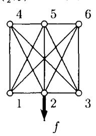
Figurc 4: A 3 x 2 grid with cxtcrnal forcc in nodc 2.
nodes are nurnbered as indicated.
By way of exarnple, let us compute vector 812, assurning x : 100. This bar's end nodes are I and 2, whose coordinates are (0,0) and (],0) respectively. Since the Iength of this bar is l/2, using (15) we find
\[\beta_{12} = \sqrt{100} \times \frac{1}{\left(\frac{1}{2}\right)^2} \begin{pmatrix} \frac{1}{2} \\ 0 \end{pmatrix} = \begin{pmatrix} 20 \\ 0 \end{pmatrix}.\]
We can forrn the vector b12, zrs defined by (16). For thc rnoment we assurne that all nodes are freel Then b12 is the first vector in the scherne below. Note that node I is fixed, hence, arcording to the definition in (16), the corresponding (first two) entries of b12 should be removed. We will deal with this later, sirnply by removing all entries in the rows corresponding to fixed nodes.
Assuming that all nodes are free, the matrix consisting of all column vectors b,,
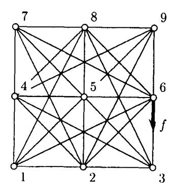
Figure 6: A \(3 \times 3\) grid with external force in node 6.
Using (26) we construct the optimal solution of the nonlinear model, which gives (with w = 1):
\[t = \left(0, 0, 0, \frac{1}{2}, 0, 0, 0, \dots, 0, 0, \frac{1}{2}, 0, 0, 0, 0, 0\right)^{T}\] and
\[\begin{split} \Delta V = - ( \ 0.1242, 0.2777, 0.2091, 0.5351, 0, 0.1946, \\ 0, 0.6250, -0.1246, 0.2775, -0.2093, 0.5352)^T. \end{split}\]
¿From this we can compute the compliance:
\[\text{Compl}_f(t) = \frac{1}{2} f^T \Delta V = \frac{1}{2} \times (-10) \times (-0.6250) = 3.1250.\]
The corresponding truss is shown left in Figure 7. Among trusses based on an \(p \times q\)
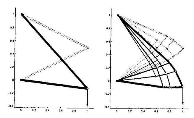
Figure 7: Trusses based on (a) \(3 \times 3\) and (b) \(21 \times 17\) grid.
grid, with \(2 \le p \le 21\) and \(3 \le q \le 21\) (q odd), the \(21 \times 17\) grid gives the lowest compliance, namely 2.9594. The corresponding truss is shown at the right in Figure 5. The next best grid is \(19 \times 19\), with compliance 2.9599.
an gri 5.
cor
Ve situ 2-d the and equ
j = 4 a (24
and
\[\Delta V = (0, -0.5062, 0.0597, -0.2049, 0, -0.2812, -0.0615, -0.2068)^T\].
lFrom this we can compute the compliance:
Complf(t) = \[\frac{1}{2}f^T \Delta V = \frac{1}{2} \times (-10) \times (-0.5062) = 2.5312\].
The corresponding truss is shown left in Figure 5. It may be clear that lower compli-
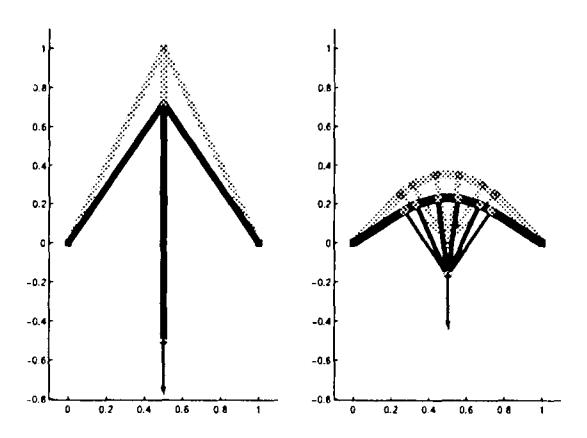
Figurc 5: TYusscs bascd on (a) 3 x 2 and (b) 17 x 21 grid
ances may be expected when using a finer grid. For example, when using a 17 x 2l grid the compliance is 0.8359; the corresponding truss is shown at the right in Figure 5. Arnong trusses based on an p x qgrid, with 3 S p < 2l (p odd) and 2 ( q < 21, the 17 x 2l grid gives the lowest compliance. The next best grid is 17 x 20, with compliance 0.8376.
Vertical load at one vertical wall In our second example we consider the situation where a vertical load has to be carried by one vertical wall, by using a (flat 2-dimensional) truss that is fixed to one side of the wall. As before, we assurne that the height and the width of the truss are I rneter, that the acting force is 10 Newtorr and that an arnount of I unit of material is available. Sc'e Figure 6, which shows an equidistant 3 x 3 grid for this problem; the vertices are given tV (i, *), i :0,1,2 and j = 0, l,2. The nodes are numbered as indicated. The fixed nodes are numbered l, 4 and 7, and the force is acting in node 6, as indicated. The solution of the problem (24) is as follows:
\[q = \left(0, 0, 0, -\frac{5}{4}, 0, 0, 0, \cdots, 0, 0, \frac{5}{4}, 0, 0, 0, 0\right)^T\] and the solution of (23) is given by
\[\Delta V = -(0.0497, 0.1111, 0.0836, 0.2140, 0, 0.0778, 0, 0.2500, -0.0498, 0.1110, -0.0837, 0.2141)^{T}.\]
given by
\[\text{[rumus tidak dapat ditampilkan dengan baik — lihat PDF asli]}\]
Note that if the two vertical components in \(f_1\) were zero, then an optimal truss would only use the two horizontal bars, both with half of the total volume w. But such a truss would not be able to carry the vertical components of the forces in the right nodes, and it would crash. Mathematically this means that then the problem (24) is infeasible, and problem (23) unbounded. In the present case the optimal solution of these problems are respectively given by
\[q^{\star} = \begin{pmatrix} 1\\0\\0.0010\\0\\0.0005\\0.9995 \end{pmatrix}, \qquad \Delta V^{\star} = \begin{pmatrix} 0.1\\0\\0.1\\0.1 \end{pmatrix}.\]
Using (26) we derive from this the optimal solution of (22), with w=1 and \(\|q^*\|_1=2.001\), which gives
\[t = \frac{1}{2.001} \begin{pmatrix} 1\\0\\0.0010\\0\\0.0005\\0.9995 \end{pmatrix}, \qquad \Delta V = 2.001 \begin{pmatrix} 0.1\\0\\0.1\\0.1 \end{pmatrix}\] and \(\text{Compl}_{f_1}(t) = \frac{1}{2} f_1^T \Delta V = 2.0020005\). Figure 10 shows the optimal truss in the unloaded and loaded case, respectively.
The optimal truss is designed for the given load. One may wonder how it behaves when it is loaded with an occasional load that differs not too much from the design load. We will demonstrate below that very small perturbations in the load may have a disastrous effect on the compliance. To make this clear, let g be an eigenvector of A(t) with eigenvalue \(\lambda\). So we have \(A(t)g = \lambda g\). Let f denote the design load of the truss and \(\Delta V\) the corresponding displacement. Without loss of generality we assume that \(\|g\| = \|f\|\) and \(f^T g \geq 0\). Now consider the situation that the design load is replaced by
\[f(\gamma) = f + \gamma g\] for some \(\gamma \geq 0\). Then the displacement \(\Delta V(\gamma)\) under the load follows by solving the equation \(A(t)\Delta V(\gamma) = f + \gamma g\), which gives
\[\Delta V(\gamma) = \Delta V + \frac{\gamma}{\lambda} g.\]
od tr
τ
ci of a of tl un an re th is 3. By tw an th
Uniformly loaded bridge In our third exarnple we want to design a bridge that crosses a river. The bridge rests on the shores of the river a"nd it has to carry a load of l0 N, which is assumed to be uniformly distributed over the whole bridge- We use 6px q grid, with the lower left and lower right node fixed, and with external forces of size l0/(q - 2) in the remaining lower nodes of the grid. As before, we assume that the height and the width of the truss are I meter. and that an atnount of I unit of material is available. Since the solution t of problem is proportional to the amount of material the sizes of the bars in the truss can be easily a.dapled to more realistic values. A similar argument applies to the chosen size of the forces acting on the bridge and to the size of the grid.
For a 6 x 21 grid the corresponding solution is shown left in Figure 8. Its compliance is 0.5000. Among trusses ba^sed on an p x g grid, with 3 < p S 21 and J < q < 2l (q
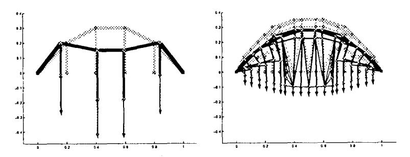
Figurc 8: tusscs bascd on (a) 6 x 21 and (b) 21 x 21 grid.
odd), the 21 x27 grid gives the lowest compliance, namely 0.3601. The corresponding truss is shown at the right in Figure 8.
3.1.7 Instability with respect to additional loads
By way of example we consider a very simple truss, based ot a2 x 2 square grid, for which the left nodes are fixed, and with external forces in the two right nodes. The two external forces have a horizontal component 10, and vertical cornporrents 0.005 and -0.005 in the upper and lower right node respeclively. The situation is depicted in Figure 9. The nodes are numbered as indicated. The rnatrix B (for rc = 100) and
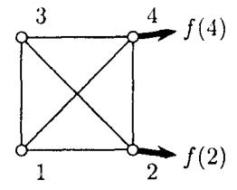
Figurc 9: A 2 x 2 grid with external forces in nodes 2 and 4.
the vector f : fr, with the entries corresponding to the fixed nodes removed, are
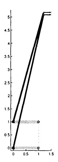
Figure 11: Instability of the truss w.r.t small occasional load.
which amounts to only 0.25% of the design load size \(||f_1||\); the new compliance value is 2.12047, which means an increase of 6%.
It is clear from the above example that small eigenvalues of the matrix A(t) may give rise to instability of the truss: a small perturbation of the load may cause a large increase of the compliance. Thus we may conclude that for a stable truss the eigenvalues of the matrix A(t) should be bounded well away from zero.
Recall from (19) that the bar-stiffness matrix A(t) was given by
\[A(t) = B \operatorname{diag}(t) B^{T} = \sum_{\{v,w\} \in \mathcal{A}} t_{vw} b_{vw} b_{vw}^{T} = \sum_{i=1}^{n} t_{i} b_{i} b_{i}^{T},\] where B denotes the node-bar matrix of the truss and t the bar-volume vector of the truss. The equation (18) will have a unique solution only if A(t) > 0. This together with the above observations more than justifies the following assumption, which we assume to be satisfied in the sequel.
Assumption 3.3 If \[t_i > 0\] for \(i = 1, ..., n\), then \(A(t) > 0\).
Note that this is also a physically meaningful assumption. It excludes rigid body motions of the ground structure: if all rigidities are positive then the potential energy stored by the structure under any nontrivial displacement is strictly positive.
3.2 Multi-load and robust versions of the TTD problem
In the previous sections we managed to derive a linear model for the TTD problem which turned out to be equivalent to the earlier proposed nonconvex quadratic model. A enlightening explanation of this very pleasant phenomenon is given in [8]. The explanation is based on a conic quadratic model of the TTD problem; this model
tl if lt:
Fr
Fo
\(\mathbf{F}\mathbf{i}\)
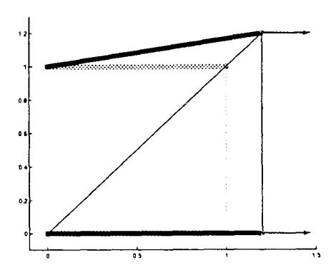
Figure 10: The optimal truss, unloaded (grey) and loaded (black).
The new compliance is then given by
\[\operatorname{Compl}_{f(\gamma)}(t) = \frac{1}{2} \left( f + \gamma g \right)^{T} \left( \Delta V + \frac{\gamma}{\lambda} g \right) \ge \operatorname{Compl}_{f}(t) + \frac{\gamma^{2}}{2\lambda} \|f\|^{2}.\]
Here we used that \(f^Tg \ge 0\) (and hence also \(g^T\Delta V \ge 0\)) and \(g^Tg = \|f\|^2\). We see that the effect on the the compliance of such a perturbation of the load may be large if the eigenvalue is small. In our case, the bar-stiffness matrix A(t) is given by
\[A(t) = B \operatorname{diag}(t)B^{T} = \frac{1}{2.001} \begin{bmatrix} 100 & 0 & 0 & 0\\ 0 & 0.05 & 0 & -0.05\\ 0 & 0 & 99.975 & 0.025\\ 0 & -0.05 & 0.025 & 0.075 \end{bmatrix}.\](29)
Its smallest eigenvalue is 0.00548, and a corresponding eigenvector g such that ||g|| = ||f|| and \(f^T g \ge 0\) is given by
\[g = ||f|| (0.00000, 0.78819, -0.000154, 0.61544)^T\].
From this we derive that
\[\operatorname{Compl}_{f(\gamma)}(t) \ge \operatorname{Compl}_{f}(t) + 18259 \gamma^{2}.\]
For \(\gamma=0.025\) (which amounts to a perturbation of 2.5%) the compliance becomes more than 13. For \(\gamma=0.0025\) the perturbed load becomes
\[f_2 = \frac{2}{4} \begin{bmatrix} 10.000000 \\ 0.022867 \\ \hline 9.999995 \\ 0.031759 \end{bmatrix} . \tag{30}\]
Figure 11 shows the loaded truss under \(f_2\). The perturbation of the load is \(\gamma ||g||\),
Lemma 3.4 Compl<sub>t</sub>\((t) \le \tau\) holds if and only if
\[\frac{1}{2}\Delta V^T A(t)\Delta V - f^T \Delta V + \tau \ge 0, \quad \forall \Delta V.\]
Proof: By (32), Compl<sub>f</sub>(t) \(\leq \tau\) is equivalent to
\[\sup_{\Delta V \in \mathbf{R}^m} \left[ f^T \Delta V - \frac{1}{2} \Delta V^T A(t) \Delta V \right] \le \tau.\]
Clearly, this holds if and only if the quadratic form
\[\frac{1}{2}\Delta V^T A(t)\Delta V - f^T \Delta V + \tau\] is nonnegative for all \(\Delta V \in \mathbf{R}^n\).
Theorem 3.5 Compl<sub>f</sub>(t) \(\leq \tau\) holds if and only if
\[\begin{pmatrix} 2\tau & f^T \\ f & A(t) \end{pmatrix} \succeq 0.\]
Proof: This immediately follows from Lemma 3.4 and Lemma A.1.
3.2.2 Semidefinite model for the multi-load TTD
The semidefinite representation of the compliance, as given by Theorem 3.5, enables us to formulate the TTD problem as a socalled semidefinite optimization problem:
\[\min_{\tau,t} \left\{ \tau : \begin{pmatrix} 2\tau & f^T \\ f & \sum_{i=1}^n b_i t_i b_i^T \end{pmatrix} \succeq 0, \quad \sum_{i=1}^n t_i \le w, \ t \ge 0 \right\}.\] (33)
In the multi-load case we assume that that the set \(\mathcal{F}\) of loading scenarios is a finite set,
\[\mathcal{F} = \{f_1, \dots, f_k\}.\]
A big advantage of the above model is that it can be easily adapted to obtain a TTD that can withstand the loads \(f_i\) in \(\mathcal{F}\) (not acting at the same time) in the best possible way.
\[\min_{\tau,t} \left\{ \tau : \begin{pmatrix} 2\tau & -f_j^T \\ -f_j \sum_{i=1}^n b_i t_i b_i^T \end{pmatrix} \succeq 0, \ j = 1, \dots, k, \sum_{i=1}^n t_i \le w, \ t \ge 0 \right\}.\] (34)
The design variables are \(t_i \in \mathbf{R}_+\), i = 1, ..., n, and \(\tau \in \mathbf{R}\). Indeed, the linear matrix inequalities (LMI's) in (34) express the fact that the worst, over the loads \(f_1, ..., f_k\), compliance of the construction yielded by the rigidities \(t_1, ..., t_n\) does not exceed \(\tau\), while the linear constraints express the fact that \(t = (t_1, ..., t_n)\) is an admissible design.
A crucial question is, of course, if we can solve these models efficiently! The answer is affirmative, as has become clear in Section 3.2.3.
p la lo
T in
3. Gi
Sir fur var
\(\frac{No}{th\epsilon}\)
Thi tha min pow tand
\(-\frac{1}{2}\)
Not
Asε can be easily extended to the multi-load case. But only in the single-load case it naturally shrinks down to a linear model. This suggests that whenever a truss has to be designed that can withstand a finite set of (more than one) loads a linear model will not suffice.
In this section we consider the multi-load case, i.e. the case where we want to design a truss that is able to withstand a finite set of different loads in the best possible way. We show that an optimal truss can be obtained by solving a semidefinite minimization problem. Robust designs are obtained by allowing the set of loads to be infinitely large, but where the set is of a special form. Below we deal with ellipsoidal sets of loads. It will turn out that this case can also be modelled by a simple minimization problem, with only one semidefinite constraint.
The models in this section are based on a simple variational principle that will be introduced in the next section.
3.2.1 Variational Principle
Given a truss t and an external load f we define the potential energy \(E_{t,f}(\Delta V)\) of the loaded system as a function of the displacement \(\Delta V\) as follows:
\[E_{t,f}(\Delta V) = \frac{1}{2} \Delta V^T A(t) \Delta V - f^T \Delta V\]
= \(\frac{1}{2} \Delta V^T B \operatorname{diag}(t) B^T \Delta V - f^T \Delta V.\) (31)
Since \(t \geq 0\), the matrix A(t) is positive semidefinite, and hence \(E_{t,f}(\Delta V)\) is a convex function. As a consequence, this function is bounded below if and only if its gradient vanishes for some \(\Delta V\), i.e., if and only of there exists \(\Delta V\) such that
\[A(t) \Delta V = f\].
Note that this is exactly equation (18), the equation for equilibrium. Thus we obtain the following Variational Principle:
The equilibrium displacement of a truss t under an external load f is a minimizer of the quadratic form
\[\frac{1}{2} \Delta V^T A(t) \Delta V - f^T \Delta V\] in the displacement \(\Delta V\); if this quadratic form is unbounded below, there is no equilibrium at all.
This is a typical variational principle in mechanics and physics. Such principles state that equilibria in certain physical systems occur at critical points (in good cases at minimizing points) of certain energy functionals. Variational principles are extremely powerful; in mechanical, electrical and other applications an issue of primary importance is to identify a tractable variational principle governing the model.
Note that in equilibrium, the (minimal) value of the energy function is given by \(-\frac{1}{2}f^T\Delta V\). Thus, using (21), we obtain
\[-\operatorname{Compl}_{f}(t) = \min_{\Delta V} \left( \frac{1}{2} \Delta V^{T} A(t) \Delta V - f^{T} \Delta V \right). \tag{32}\]
As a consequence we have the following lemma, which needs no further proof.
For \(\gamma = 0.01\) the perturbed load becomes
\[f_3 = \begin{pmatrix} 2 \\ 4 \end{pmatrix} \begin{bmatrix} 10.000000 \\ -0.127949 \\ \hline 10.000192 \\ -0.059882 \end{bmatrix} . \tag{36}\]
Figure 13 shows the loaded truss under \(f_3\); The increase in the load size is \(\gamma ||g||\),
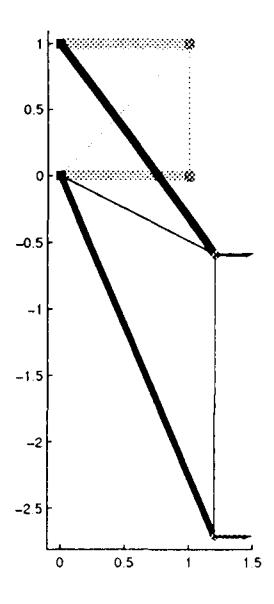
Figure 13: Instability of the multi-load truss w.r.t small occasional load.
which amounts to only 1% of the design load size ||f||; the new compliance value is 2.25312, which means an increase of about 12.5%.
3.2.4 The robust TTD problem
We finally consider the so called robust TTD problem, where we assume that the set of loads \(\mathcal{F}\) is an ellipsoid:
\[\mathcal{F} = \left\{ f = Qu : u^T u \le 1 \right\}, \quad Q \in \mathbf{M}^{m \times p}. \tag{37}\]
The matrix Q has to be chosen such that the ellipsoid \(\mathcal F\) contains all possible loads that the truss has to withstand. Since the set \(\mathcal F\) is infinite, we meet a difficulty not present in the case of finite \(\mathcal F\), namely that the objective now is to minimize
\[\operatorname{Compl}_{\mathcal{F}}(t) = \sup_{f \in \mathcal{F}} \operatorname{Compl}_{f}(t), \tag{38}\] which is the supremum of infinitely many SDR function. Fortunately, it is nevertheless easy to get an SDR for \(Compl_{\mathcal{F}}(t)\).
Figure and
Ua loa tri de and prob truss this l
small for w For th
ing (n
Using with \(\gamma\)
3.2.3 Example of a multi-load truss
We turn back to the problem considered in Section 3.1.7. In that section we considered the single load truss for the design load \(f_1\), and we also subjected the resulting truss to the load \(f_2\), as given by (30). Thus these forces are given by
\[f_1 = \frac{2}{4} \begin{bmatrix} 10.000000 \\ -0.005000 \\ 10.000000 \\ 0.010000 \end{bmatrix}, \qquad f_2 = \frac{2}{4} \begin{bmatrix} 10.000000 \\ 0.022867 \\ 9.999995 \\ 0.031759 \end{bmatrix}. \tag{35}\]
Using the same grid as there, we can now optimize the truss with respect to both loads by solving (34) for k = 2 and \(f_1\) and \(f_2\) as just given. The optimal multi-load truss t with respect to these loads, when loaded with one of these loads, behaves as depicted in Figure 12. The compliance of the truss with respect to \(f_1\) is 2.012455,
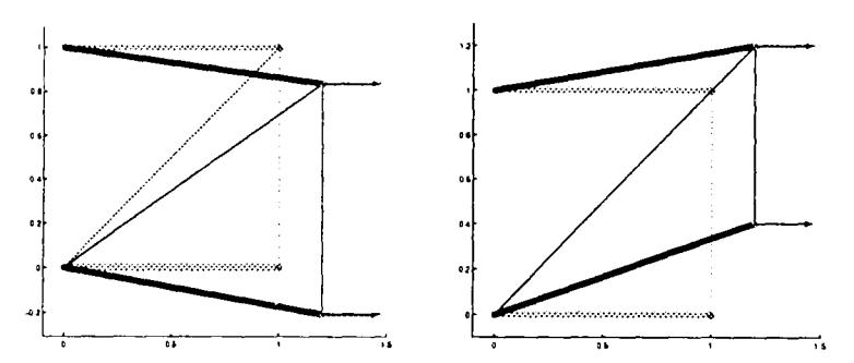
Figure 12: Multi-load truss subjected to the two separate design loads \(f_1\) (left) and \(f_2\) (right).
and with respect to \(f_2\) is the compliance 2.015527 (which is also the optimal value of problem (34). Comparing the right figure in Figure 12 with the behavior of the single truss load under \(f_2\), as depicted in Figure 11, we see that the new truss withstands this load considerably better.
Note that this result does not imply that the new truss is stable with respect to other small perturbations of the load. In fact, this is not the case. To obtain a perturbation for which the truss is most sensitive we use the same approach as in Section 3.1.7.
For the new truss the smallest eigenvalue of A(t) is \(\lambda = 0.049163\) and the corresponding (normalized) eigenvector g such that \(||g|| = ||f_1||\) and \(f_1^T g \ge 0\) is given by
\[g = ||f_1|| (0.00000, -0.86938, 0.00135, -0.49413)^T.\]
Using the notation of Section 3.1.7, we replace the design load by
\[f(\gamma) = f_1 + \gamma g,\] with \(\gamma \geq 0\). Then the compliance with respect to \(f(\gamma)\) satisfies
\[\operatorname{Compl}_{f(\gamma)}(t) \geq \operatorname{Compl}_{f_1}(t) + \frac{\gamma^2}{2\lambda} \|f_1\|^2 \approx \operatorname{Compl}_{f_1}(t) + 2034 \,\gamma^2.\]
| 1 | LO (lL) | sDo (2L) | sDo (3L) | SDO (Rob.) | |
|---|---|---|---|---|---|
| 2 | ttz | 0.4998 | 0.4981 | 0.4876 | 0.4576 |
| J | rl3 | 0 | 0 | 0 | 0 |
| i | tra | 0.0005 | 0.0054 | 0.0007 | 0.0377 |
| o | .23 | 0 | U | 0.0156 | 0.0377 |
| 6 | 124 | 0.0002 | 0.001l | 0.0024 | 0.0093 |
| '7 | 0.4995 | 0.4954 | 0.4937 | 0.4576 | |
| 8 | Design Cornpl. | 2.0020 | 2.0155 | 2.0519 | 2.1 63 1 |
| I | Compl. w.r.t /1 | 2.0020 | 2.0125 | 2.0378 | 2.1548 |
| l 0 | Compl. w.r.t f2 | 2.1205 | 2.0155 | 2.0155 | 2.1560 |
| l l | Cornpl. w.r.t /3 | 3.7790 | 2.2531 | 2.0519 | 2.1 609 |
| t 2 | );1,, (A(r)) | 182.5928 | 20.3405 | 17.2258 | 1.0820 |
Figurc 14: Optimal trusses and thcfu compliances.
both loads. The obtained truss turned out to be instable with respect to the load /3, as defined bV (36). The just mentioned results of these sections are summarized in the second and third column of the table in Figure 14.
The rows 2-7 give the volumes of the bars, row 8 the value of the cornpliance for the design, and rows 9-ll the actual compliance with respect to the loads /1, /2 and /3 respectively. The last row gives the inverse of the srnallest eigenvalue of the bar-stiffness matrix A(t); we already have seen that this quantity can be considered 3^s a rne&sure f<rr the robustness of the trus.
The fourth column in the table gives the corresponding values for the rnulti-load model (34) where the loads are now /1, f2 and. /3. It is depicted left in Figure l5 under the three given loads.
F
T
T so
Nr sh 3. In wl re un us
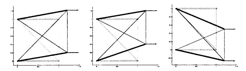
Figurc 15: Multi-load truss loaded with fi (left), with /2 (middlc) and /3 (right).
Finally, in the fifth column one finds the solution of the robust sernidefinite model
Theorem 3.6 Let \(\mathcal{F}\) be as given by (37). Then one has one has \(\operatorname{Compl}_f(t) \leq \tau\) for each \(f \in \mathcal{F}\) if and only if
\[\begin{pmatrix} 2\tau I_p & Q^T \\ & & \\ Q & \sum_{i=1}^n b_i t_i b_i^T \end{pmatrix} \succeq 0.\]
Proof: With \(Compl_{\mathcal{F}}(t)\) as defined by (38), we may write
\[\begin{aligned} \operatorname{Compl}_{\mathcal{F}}(t) &\leq \tau \Leftrightarrow \frac{1}{2} x^T A(t) x - (Q u)^T x + \tau \geq 0, \ \forall x \ \forall (u \ : \ u^T u \leq 1) \\ &\Leftrightarrow \frac{1}{2} x^T A(t) x - (Q u)^T x + \tau \geq 0, \ \forall x \ \forall (u \ : \ u^T u = 1) \\ &\Leftrightarrow \frac{1}{2} x^T A(t) x - (Q \frac{u}{\|u\|})^T x + \tau \geq 0, \ \forall x \ \forall u \neq 0 \\ &\Leftrightarrow \frac{1}{2} (\|u\| x)^T A(t) (\|u\| x) - (Q u)^T (\|u\| x) + \tau u^T u \geq 0, \\ \forall x \ \forall u. \end{aligned}\]
Replacing ||u|| x by -y we obtain
\[\begin{aligned} \operatorname{Compl}_{\mathcal{F}}(t) &\leq \tau \Leftrightarrow 2\tau u^T u + 2u^T Q^T y + y^T A(t) y \geq 0, \quad \forall y \ \forall u \\ &\Leftrightarrow \begin{pmatrix} u \\ y \end{pmatrix}^T \begin{pmatrix} 2\tau I_p \ Q^T \\ Q \ A(t) \end{pmatrix} \begin{pmatrix} u \\ y \end{pmatrix} \geq 0, \quad \forall y \ \forall u \\ &\Leftrightarrow \begin{pmatrix} 2\tau I_p \ Q^T \\ Q \ A(t) \end{pmatrix} \succeq 0. \end{aligned}\]
For the last equivalence we used again Lemma A.1. This proves the theorem.
Theorem 3.6 enables us to model the robust TTD problem as follows:
\[\min_{\tau, t} \left\{ \tau : \begin{pmatrix} 2\tau I_p & Q^T \\ Q & \sum_{i=1}^n b_i t_i b_i^T \\ \end{pmatrix} \succeq 0, \quad \sum_{i=1}^n t_i \leq w, \ t \geq 0 \right\}.\] (39)
This model finds the truss which is best able to withstand all the loads in the ellipsoidal set of loads
\[\mathcal{F} = \left\{ f = Qu : u^T u \le 1 \right\}, \quad Q \in \mathbf{M}^{m \times p}.\]
Note that it does not tell us how to choose the matrix Q. But it is clear that we should choose Q in such a way that the ellipsoid \(\mathcal{F}\) contains all loads that may occur.
3.2.5 Examples of robust designs
In this final section we consider again the \(2 \times 2\) grid of Figure 9 in Section 3.1.7, which was also used in Section 3.2.3. In Section 3.1.7 we found the truss optimal with respect to \(f_1\) by solving the linear model (24); it turned out that this truss is very unstable with respect to the load \(f_2\) (cf. (35)). Subsequently, in Section 3.2.3, we used the multi-load semidefinite model (34) to find the optimal truss with respect to
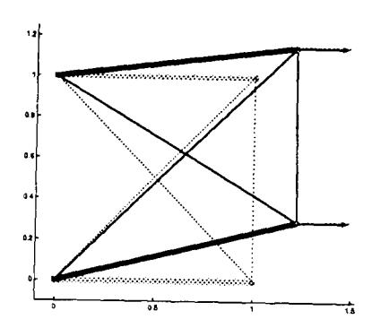
Figure 17: The robust truss w.r.t a small occasional load.
structure. Then (34) is a semidefinite problem with design dimension n+1, \(n=O(M^2)\) being the number of tentative bars. The problem contains k (k is the number of loading scenarios) big LMI's (each of the row size m+1, where m is the number of degrees of freedom of the nodal set; \(m\approx 2M\) for planar and \(m\approx 3M\) for spatial trusses) and n+1 linear inequality constraints.
For a planar \(15 \times 15\) grid with the left nodes fixed, we get M = 225, n+1 = 25096, m = 420. Even an LP problem with 25.000 variables should not be treated as a small one; a semidefinite problem of such a huge dimension is definitely not accessible for existing software.
The situation, however, is not hopeless, and the way to overcome the difficulty is offered by duality. The dual problems of (34) and (39) can be greatly simplified by analytical elimination of most of their variables. For example, the dual to the outlined multi-load truss problem can be converted to a semidefinite problem with nearly mk design variables; for the \(15 \times 15\) ground structure and three scenarios, its design dimension is about 1300, which is within the range of applicability of existing solvers.
Below we will show how this can be reached for the multi-load problem; similar arguments can be applied to the robust problem. The outcome of the process will be summarized, for both cases, in Section 3.3.5. Note that (34) can be restated as
\[\min_{\tau,t} \left\{ \tau : \begin{pmatrix} 2\tau & f_j^T \\ f_j & \sum_{i=1}^n b_i t_i b_i^T \end{pmatrix} \succeq 0, \ j = 1, \dots, k, \sum_{i=1}^n t_i \le w, \ t \ge 0 \right\}.\] (41)
The only change is that we replaced \(f_j\) by \(-f_j\) in the LMIs; this makes no difference and is more convenient for our purpose.
3.3.1 Building the dual
We introduce dual matrix variables
\[\left(\begin{array}{cc} \alpha_j & v_j^T \\ v_j & \beta_j \end{array}\right) \succeq 0\]
\(C_{i}\)
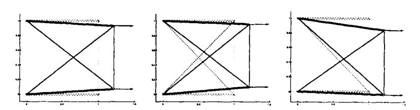
Figure 16: Robust truss loaded with \(f_1\) (left), with \(f_2\) (middle) and \(f_3\) (right).
(39) for the matrix
\[Q = \left(\begin{array}{ccc} 10 & 0 & 0 \\ 0 & 2 & 0 \\ 10 & 0 & 0 \\ 0 & 0 & 2 \end{array}\right).\]
This means that the obtained truss is optimal with respect to the ellipsoidal set of loads
\[\mathcal{F} = \left\{ f = Qu = \begin{pmatrix} 10u_1 \\ 2u_2 \\ 10u_1 \\ 2u_3 \end{pmatrix} : u \in \mathbf{R}^3, u^T u \le 1 \right\}.\]
It is depicted left in Figure 16 under the three given loads. From the table it is clear that the inverse of the smallest eigenvalue of the bar-stiffness matrix is by far the smallest when compared with the other trusses. This means that the truss should be much more stable than the other trusses when loaded with any small occasional load. To verify this we conclude this section by loading this truss with a load of the form \(f_1 + \gamma g\), where g is a unit eigenvector of the bar-stiffness matrix for its smallest eigenvalue. The smallest eigenvalue of A(t) is \(\lambda = 0.924217\) and the corresponding eigenvector g such that \(\|g\| = \|f_1\|\) and \(f_1^T g \geq 0\) is given by
\[g = ||f_1|| (0.01457, 0.70696, -0.01457, 0.70695)^T\].
For \(\gamma = 0.02\) the perturbed load becomes
\[f_4 = \frac{2}{4} \begin{bmatrix} 10.004122\\ 0.194958\\ 9.995878\\ 0.209958 \end{bmatrix}. \tag{40}\]
Figure 17 shows the loaded truss under \(f_4\); The increase in the load size is \(\gamma ||g||\), which amounts to 2% of \(||f_1||\); the new compliance value is 2.19915.
3.3 Simplifying the semidefinite models by using duality
A disadvantage of the semidefinite models (34) and (39) is their huge dimension. Consider, for example, in the multi-load case (34) a truss with an M-node ground
Hence, the inequalities (a) and (d) imply the inequality
\[\sum_{j=1}^k b_i^T v_j \alpha_j^{-1} v_j^T b_i \le \gamma, \quad i = 1, \ldots, n.\]
On the other hand, if the last inequality holds, taking \(\beta_j = v_j \alpha_j^{-1} v_j^T\), also (a) and (d) follow. Thus we conclude that the following problem has the same optimal value as (43).
supremum \[-2\sum_{j=1}^{k} f_{j}^{T} v_{j} - w\gamma\] such that \[(b) \qquad \gamma \geq 0,\] \[(c) \qquad 2\sum_{j=1}^{k} \alpha_{j} = 1,\] \[(d') \qquad \sum_{j=1}^{k} b_{i}^{T} v_{j} \alpha_{j}^{-1} v_{j}^{T} b_{i} \leq \gamma, \quad i = 1, ..., n,\] \[(e) \qquad \alpha_{j} > 0, \quad j = 1, ..., k.\] \[(44)\]
Due to (e), and by the Schur complement lemma, the system of inequalities (d') is equivalent to the following system of LMIs:
\[\begin{pmatrix} \alpha_1 & & & v_1^T b_i \\ & \ddots & & \vdots \\ & & \alpha_k & v_k^T b_i \\ \hline b_i^T v_1 & \dots & b_i^T v_k & \gamma \end{pmatrix} \succeq 0, \quad i = 1, \dots, n, \tag{45}\]
Consequently, we may replace the constraints (d') in problem (44) by (45). Note that (45) implies \(\alpha_i \geq 0\), for all i. Hence, since our problem is still strictly feasible, omitting constraint (e) in (44) does not change the optimal value. Also note that (45) implies \(\gamma \geq 0\), i.e. constraint (b) in (44). Thus we arrive at the final form of our dual problem of (41):
maximus \[-1 \sum_{j=1}^{n} \frac{1}{3_{j}} v_{3} - w_{3}\] such that \[\text{[rumus tidak dapat ditampilkan dengan baik — lihat PDF asli]}\] \[(46)\] \[(b) \qquad \qquad 2 \sum_{j=1}^{k} \alpha_{j} = 1,\]
We already established that both the primal problem (41) and its dual problem (46) are strictly feasible. Consequently, both problems are solvable and their optimal values equal.
3.3.4 Back to primal
Problem (46) is not exactly the dual of (41) – it is obtained by elimininating part of the variables. What happens if we pass from (46) to its dual? It turns out that 3.
pro
It is we made the Chocolarge feasily value
3.3.3
Since interior value. constr for the LMIs in (41), with \(\alpha_j \in \mathbf{R}\), \(\beta_j \in \mathbf{S}^m\), \(v_j \in \mathbf{R}^m\), and dual scalar variables \(\gamma \in \mathbf{R}_+\) for the weight constraint and \(\tau_i \in \mathbf{R}_+\) for the nonnegativity constraints. The dual problem is then given by maximize \[-2\sum_{j=1}^{k} f_{j}^{T} v_{j} - w\gamma\] such that \[\begin{pmatrix} \alpha_{j} & v_{j}^{T} \\ v_{j} & \beta_{j} \end{pmatrix} \succeq 0, \quad j = 1, \dots, k,\] \[(b) \qquad \qquad \gamma \geq 0,\] \[(c) \qquad \qquad \tau_{i} \geq 0, \quad i = 1, \dots, n,\] \[(d) \qquad \qquad 2\sum_{j=1}^{k} \alpha_{j} = 1,\] \[(e) \qquad \sum_{j=1}^{k} b_{i}^{T} \beta_{j} b_{i} + \tau_{i} - \gamma = 0, \quad i = 1, \dots, n,\] \[(42)\]
3.3.2 Eliminating the \(\tau_i\)'s
It is obvious that we can eliminate the slack variables \(\tau_i\), thus arriving at the equivalent problem
maximize \[-2\sum_{j=1}^{k} f_{j}^{T} v_{j} - w \gamma\] such that \[(a) \qquad \begin{pmatrix} \alpha_{j} & v_{j}^{T} \\ v_{j} & \beta_{j} \end{pmatrix} \succeq 0, \quad j = 1, \dots, k,\] \[(b) \qquad \qquad \gamma \geq 0,\] \[(c) \qquad \qquad 2\sum_{j=1}^{k} \alpha_{j} = 1,\] \[(d) \qquad \qquad \sum_{i=1}^{k} b_{i}^{T} \beta_{j} b_{i} \leq \gamma, \quad i = 1, \dots, n,\] \[(43)\]
It is worth noting that (43), and as a consequence also (42), is strictly feasible. Indeed, we may choose arbitrary positive reals \(\alpha_j\) and by normalization, we may enforce (c). Choosing \(\beta_j\) large enough we enforce strict inequality in (a). Finally, choosing \(\gamma\) large enough also (d) will hold strictly. Since the primal problem (41) is also strictly feasible, we conclude that both problems have optimal solutions and that the optimal values are equal!
3.3.3 Eliminating the \(\beta_j\)'s
Since (43) is strictly feasible, when adding the constraints \(\alpha_j > 0\), for all j, the interior of the feasible region does not change, and hence neither does the optimal value. However, if \(\alpha_j > 0\) then we may apply the Schur complement lemma to the constraints in (a), yielding the equivalent constraints
\[v_j \alpha_j^{-1} v_j^T \preceq \beta_j, \quad j = 1, \ldots, k.\]
To prove the converse part of the theorem, let \((t_1, \ldots, t_n, \tau)\) be feasible to (41). As before we fix \(j, 1 \leq j \leq k\). For every \(x \in \mathbf{R}\) the quadratic form (48) of \(y \in \mathbf{R}^m\) is nonnegative, hence bounded below. The minimizer of this form satisfies
\[A(t)y = -xf_j \qquad \left[ A(t) = \sum_{i=1}^n b_i t_i b_i^T \right]\] and hence this equation is solvable for every x. This holds in particular if x = -1. Let the vector \(y_j\) satisfy
\[A(t)y_j=f_j.\]
Now define
\[q_i^j = t_i b_i^T y_j. (49)\]
Į
fc
CO
Then we have
\[\sum_{i=1}^{n} q_i^j b_i = \sum_{i=1}^{n} b_i t_i b_i^T y_j = A(t) y_j = f_j,\] (50)
thus ensuring the validity of equation (c) in (47). It remains to show that the LMI's (a) in (47) are satisfied as well. Thus we finally need to show that for every \(x \in \mathbf{R}\) and for every vector \(\xi = (\xi_i)_{i=1}^n\) we have
\[F(x,\xi) \equiv 2\tau x^2 + 2\sum_{i=1}^n xq_i^j \xi_i + \sum_{i=1}^n t_i \xi_i^2 \ge 0.\] (51)
Given x, let us set
\[\xi_i^* = -xb_i^T y_j,\] and let us prove that the vector \(\xi^*\) minimizes \(F(x,\xi)\). This is easy, because F(x,.) is a convex quadratic form, and its partial derivative with respect to \(\xi_i\) at the point \(\xi_i^*\) is equal to (see (49))
\[2xq_{i}^{j} + 2t_{i}\xi_{i}^{*} = 2\left(xt_{i}b_{i}^{T}y_{j} - t_{i}xb_{i}^{T}y_{j}\right) = 0,\] for all i, proving the claim. Thus, to complete the proof of (51), we only need to show that \(F(x,\xi^*) \geq 0\). This goes as follows:
\[\begin{split} F(x,(\xi_i^*)_{i,s}) &= 2\tau x^2 + 2\sum_{i=1}^n xq_i^j\xi_i^* + \sum_{i=1}^n t_i\xi_i^{*2} \\ &= 2\tau x^2 - 2\sum_{i=1}^n x^2q_i^jb_i^Ty_j + \sum_{i=1}^n x^2y_j^Tb_it_ib_i^Ty_j \\ &= 2\tau x^2 - 2x\left(\sum_{i=1}^n q_i^jb_i\right)^Txy_j + x^2y_j^TA(t)y_j \\ &= 2\tau x^2 - 2xf_j^Txy_j + x^2y_j^TA(t)y_j. \end{split}\]
The last reduction used (50). Hence we write
\[F(x,\xi^*) = \begin{pmatrix} x \\ -xy_j \end{pmatrix}^T \begin{pmatrix} 2\tau & f_j^T \\ f_j & A(t) \end{pmatrix} \begin{pmatrix} x \\ -xy_j \end{pmatrix}\]
Since \((t_1, \ldots, t_n, \tau)\) is feasible to (41) the last expression is nonnegative, and hence the proof is complete.
we end up with a nontrivial (and instructive) equivalent formulation of (41), namely, with the problem
min \[\tau\]
s.t.
(a) \(\begin{pmatrix} 2\tau & q_1^j & \dots & q_n^j \\ \hline q_1^j & t_1 & & \\ \vdots & & \ddots & \\ q_n^j & & t_n \end{pmatrix} \succeq 0, \quad j = 1, \dots, k,\)
(b) \(\sum_{i=1}^n t_i \leq w,\)
(c) \(\sum_{i=1}^n q_i^j b_i = f_j, \quad j = 1, \dots, k,\)
where the design variables are
- \(t_i \in \mathbf{R}_+\) and \(\tau \in \mathbf{R}\);
- \(q_i^j \in \mathbf{R}, j = 1, ..., k, i = 1, ..., n\)
(47) is not the straightforward dual of (46); it is obtained from this dual by eliminating part of the variables. Instead of deriving (47) in this way, we prefer to give a direct proof of its equivalence to (41) by proving the following result.
Theorem 3.7 A collection \((t_1, \ldots, t_n, \tau)\) is feasible to (41) if and only if it can be extended by properly chosen
\[\left\{q_i^j \in \mathbf{R}^p : j = 1, \ldots, k, i = 1, \ldots, n\right\}\] to a feasible solution to (17).
Proof: Let \((t_1, \ldots, t_n, \tau)\) and
\[\left\{ q_i^j \in \mathbf{R}^p : j = 1, \dots, k, i = 1, \dots, n \right\}\]
compose a feasible solution to (47). Fixing j (\(1 \le j \le k\)), we should prove the validity of the LMIs in (41). Thus we should prove that for every pair (x, y) with \(x \in \mathbf{R}\) and \(y \in \mathbf{R}^m\) we have
\[2\tau x^{2} + 2xf_{j}^{T}y + y^{T} \left(\sum_{i=1}^{n} b_{i}t_{i}b_{i}^{T}\right)y \ge 0.\] (48)
In view of (c) in (47) the left hand side of (48) is equal to
\[2\tau x^2 + 2x\sum_{i=1}^n q_i^j b_i^T y + y^T \left(\sum_{i=1}^n b_i t_i b_i^T\right) y = 2\tau x^2 + 2\sum_{i=1}^n x q_i^j \xi_i + \sum_{i=1}^n t_i \xi_i^2,\] where \(\xi_i = b_i^T y\). The resulting expression is nothing but the value of the quadratic form with the matrix from the left-hand side of the LMI (a) in (47) at the vector comprised of x and \((\xi_i)_i\), and therefore is nonnegative, as claimed.
| Design dimension | |||
|---|---|---|---|
| (41) | n+l=0.5i12 | ||
| (46) | tr*+k+lx2kM | ||
| (47) | nk+n+l=0.5kM2 | ||
| and sizes of LMI's f | |||
| (41) | k ot (2M + l) x (2/r/ + l) | ||
| (46) | n x 0.5M2 of (,k+ t) x (ft + 1) | ||
| (47) | &of(n+1)x(z+1) | ||
| f t-rf lirrcar corrstraints | |||
| (41) | rL+7=0.5M2 | ||
| (46) | |||
with M free nodes. Note that in this case p : l, n x 0.5M2 and rn = 2M. Assuming k << M, here are the sizes of (41), ( O) and (47) :
We see that if the number ,t of loading scenarios is small (which norrnally is the case), the design dimension of the dual problem (46) is by orders of magnitude less than the design dimensions of both prirnal problems. As a kind of penalization, the dual problem involves a lot (= 0.5M2) of LMI's irrstcad of just ft LMI's in the primal problems. But the LMI's in the prirnal problems are large, and these in the dual small in size. When solving these problems with the best-known nurnerical techniques so far (the interior-point algorithms), thc computational effort for (41) is O(M6), while for (46) it is only O(k3 lvt3). For large M and small & this does rnake a significant difference!
(47) kM+l
Of course, there is an irnrncdiate concern about the dual problem: the actual design problems are not seen in it at all. IIow do we recover a (nearly) optimal construction from a (nearly) optimal solution to the dual problem? Irr frct. however, thcre is no reason to be concerned: the required recovering routines exist arrd are cheap com putat ionally.
4 Concluding remarks
In this paper we illrr^strated the use of conic optimization as a powerful tool for the mathematical modelling of inherently nonlinear problerrrs. As an exatnple we used the truss topology design problem. One rnay check the reference list below to observe that with the exception of one paper all relevant papers appeared in the lzrst 10 years. Indeed, the subject thanks its existence to the development of efficient solution rnethods for conic optimization problems in the la^st decade. Bspecially the possibility of nrodelling robustness of a design in a computationally trartable way opens the way to many new applications. We demonstrated this only for the TTD problem, which is a popular application in the literature. For other interesting applications we refer to [8] and the other references. It may be expected that the ongoing researc]t will bring forth many new importamt applications in the near future.
3.3.5 Summary of the semidefinite models for multi-load and robust TTD
In this section we summarize the results of the previous sections by presenting explicit forms of the primal (41), the simplified dual (46) and the simplified primal problem (47) for the multi-load problem, and similar versions for the robust truss design problems, respectively.
| Multi – load TTD | Robust TTD |
|---|---|
| problem | |
| \(\min \tau\) | \(\min \tau\) |
| s.t. | s.t. |
| \(\begin{pmatrix} 2\tau & f_j^2 \\ & n \end{pmatrix}\) | \(\int 2\tau I_p Q^T\) |
| \[(a) \begin{pmatrix} 2\tau & f_j^T \\ f_j \sum_{i=1}^n b_i t_i b_i^T \\ \end{pmatrix} \succeq 0, \ j=1:k,\] | \(\begin{pmatrix} (a) & \left( & Q & \sum_{i=1}^n b_i t_i b_i^T \ \right) \succeq 0, \end{pmatrix}\) |
| \[(b) \qquad \sum_{i=1}^{n} t_i \leq w,\] | \[(b) \sum_{i=1}^{n} t_i \leq w,\] |
| \[(c) t_i \geq 0, i = 1:n.\] | |
| Simplified d | ual problem |
| \[\max -2\sum_{j=1}^{k} f_j^T v_j - w\gamma\] | |
| s.t. \(\left\langle \begin{array}{cc} \alpha_1 & & \left| v_1^T b_i \right\rangle \end{array} \right\rangle\) | \[\max_{\mathbf{x}} -2\operatorname{Tr}\left(Q^TV\right) - w\gamma\] s.t. |
| \[(a) \begin{pmatrix} \ddots & \ddots & \vdots \\ \frac{\alpha_k}{b_i^T v_1 \dots b_i^T v_k} & \frac{v_k^T b_i}{\gamma} \end{pmatrix} \succeq 0, \ i = 1:n\] | \[(a) \begin{pmatrix} \alpha & V^T b_i \\ b_i^T V & \gamma \end{pmatrix} \succeq 0, \ i = 1:n,\] |
| \[2\sum_{i=1}^{k}\alpha_{j}=1.\] | (b) \(2\operatorname{Tr}(\alpha) = 1.\) \(\alpha \in \mathbf{R}^p, \ V \in \mathbf{M}^{m \times p}\) |
| Simplified | l primal |
| \(\min \tau\) | \(\min \tau\) |
| s.t. | s.t. |
| \[(a) \begin{pmatrix} \frac{2\tau}{q_1^j} & \frac{q_1^j}{t_1} & \dots & q_n^j \\ \vdots & \ddots & \vdots \\ q_n^j & & t_n \end{pmatrix} \succeq 0, \ j = 1:k,\] | 1 77 |
| \[\sum_{i=1}^{n} t_i \leq w,\] | n |
| (c) \[\sum_{i=1}^{n} b_i q_i^j = f_j, \ j = 1:k.\] | (b) \[\sum_{i=1}^{n} t_i \leq w,\] (c) \[\sum_{i=1}^{n} b_i q_i^T = Q.\] |
3.3.6 Evaluation
To understand how fruitful our effort was, it is enlightening to compare the sizes of the original problem (41) and the reformulation (46) of its simplified dual problem. Let us restrict ourselves to the simple case of a planar k-load truss design problem
- 19] A. tsen-Tal and A. Nemirovski. Stable Ttuss Topology Design via Semidefinite Programming. SIAM J. Optim., 7:991-1016, 1997.
- [10] A. Ben-'fal and A. Nemirovski. Robust solutions of Linear Programming problems contaminated with uncertain data. Mathematical Prcgramming,88:4ll-424, 2000.
- [11] A. Ben-Tal and A. Nemirovski. On tractable approximations of uncertain linear rnatrix inequalities affected by interval uncertainty. SIAM J. on Optimization. l2(3):811-833,2002.
- Il2i A. Ben-Tal and A. Nemirovski. Robust optirnization-methodology and applica-Lions. Math. Progrom.,92(3, Ser. B):453-480, 2002. ISMP 2000, Part 2 (Atlanta, GA).
- [13] A. Ben-Tal and A. Nemirovski. Potential reduction polynomial tirne met]rod for truss topolory design. SIAM J. Optim.,4(3):596-612, 1994.
- [14] L. El Ghaoui and H. Lebret. Robust solutions to leiut-square problenrs with uncertain data matrices. SIAM J. of Matri.r Anal. and Appl.,78:1035-1064, 1997.
- Il5l L. Et Ghaoui, F. Oustry, and H. Lcbret. Robust solutions to uncertain sernidefinite programs. SIAM J. Optin.,9:33-52, 1998.
- [16] L. El Ghaoui. Inversion error, condition number, and approxirnate inverses of uncertain matrices. Linear Algebra and, its Applications.343l344(2002),171-193.
- [17] F. Jarre, M. Kocvara, and J. Zowe. Optimal truss design by interior-point rncthods. SIAIi J. Optim., 8(4):1084-1107 (electrorric), 1998.
- ilSl Y. Nesterov and A.S. Nemirovski. Interior point polgnom,ial algorithms tn conue:L progratnnting SIAI\,1 Studies in Applied Mathernatics, Vol. 13. SIAM, Philadelphia, USA. 1994.
- [19] C. Roos, T. Terlak.y, and J.-Ph.Vial. Theory and Algoritlnns tor Linear Optimization. An Interior-Point Approoch. John Wiley & Sons, Chichester, UK, 1997.
- [20] N.Z. Shor. Quadratic optirnization problerns. Souiet Joutnal of Contputer and Systern Sciences, 25: l-l l, 1987.
- [2ll A.t,. Soyster. Convex Programming with Set-Inclusive Constraints and Applications to Inexact Linear Programnring. Operations Reseorch,2l:1154-1157, 1973.
- l22l T. 'ferlaky (ed.). Interior Point Methods ol Mathematical Programrning. Kluwer Academic Publishers, Dordrecht, The Netherlands, 1996.
- t23l S. J. Wright. Primal-Dual Interior-Point lvfethods. SIAM, Philadelphia, USA, 1997.
- I24l Y. Ye. Interior Point Algorithrns, Theory and Analysis. John Wiley & Sons, Chichester. UK, 1997.
- [25] J. Zowe, M. Kocvara, and M. P. Bendsse. Free material optimization via mathematical programming. Math. Progromming, 79(1-3, Ser. B):445-466, 1997.
P fc
R,
Ir
I2l
t3l
t4l
t6l
[5]
[7]
I8l
A Appendix
Lemma A.1 (Shor [20]) Let \(A \in \mathbb{R}^{n \times n}\), \(b \in \mathbb{R}^n\) and \(c \in \mathbb{R}\). Then the quadratic form \(x^T A x + 2b^T x + c\) is nonnegative for all \(x \in \mathbb{R}^n\) if and only if
\[\begin{pmatrix} A & b \\ b^T & c \end{pmatrix} \succeq 0\] or, equivalently \(\begin{pmatrix} A & -b \\ -b^T & c \end{pmatrix} \succeq 0\).
Proof: The proof consists of a sequence of logically equivalent statements, as follows:
\[\forall x : x^T A x + 2b^T x + c \ge 0 \quad \Leftrightarrow\] \[\forall (t \ne 0, x) : t^{-2} x^T A x + 2t^{-1} b^T x + c \ge 0 \quad \Leftrightarrow\] \[\forall (t \ne 0, x) : x^T A x + 2tb^T x + ct^2 \ge 0 \quad \Leftrightarrow\] \[\forall (t, x) : x^T A x + 2tb^T x + ct^2 \ge 0 \quad \Leftrightarrow\] \[\forall (t, x) : \begin{pmatrix} x \\ t \end{pmatrix}^T \begin{pmatrix} A & b \\ b^T & c \end{pmatrix} \begin{pmatrix} x \\ t \end{pmatrix} \ge 0 \quad \Leftrightarrow \quad \begin{pmatrix} A & b \\ b^T & c \end{pmatrix} \succeq 0.\]