

1 Introduction
The stacked-Josephsorr junctions we consider here consist of three slabs of superconducting material which have an insulating barrier between two superconductors. An important application of these long Josephson junctions (LJJ) is the magletic flux quanta (fluxon^s). The fluxon. *'hich is a circulating current, can move a)ong the junctions if tlrere is a biased current applied.
The one dinrensional stacked-LJJ cal be modelled b1' a perturbed sine-Cordon erluaticrn which, in nornralized form, may be nritten as [9]:
\[\phi_{xx}^{1} - \phi_{tt}^{1} - \sin \phi^{1} - S\phi_{xx}^{2} = \alpha \phi_{t}^{1} - \gamma, \phi_{xx}^{2} - \phi_{tt}^{2} + \sin \phi^{2} / J - S\phi_{xx}^{1} = \alpha \phi_{t}^{2} - \gamma.\] (1)
llere d' is tlre superconducting phase difference across tlrc jurrction r [l]. Tht' t,er:at o61 models the damping due to quasi particle tuulellirrg. o > 0. The driving force, correspouding to the normalized bias current'1, typicallv lies irr the interval 0 S f S 1. S e l-1.0] is the couplirrg parameter of the two junctions and J is the ratio of the critical current of of the two junctions.
One of the solutions of the unperturbed-sine-Gordon equation (6,, - d,, = sin d) is th€ solitolr
\[\phi_0 = 4 \arctan \left[ \exp \left( \frac{x - ct - \xi_0}{\sqrt{1 - c^2}} \right) \right]. \tag{2}\] which is moving with velocitj'c, lcl < 1. In the u;;;;"0 equation this parameter is not determined. The wave speed will become a function of 1 when o and S do not vanish arrd the damping is balanced by the driving force. Therefore, c is a function of 'y for given a & 5. The free parameter (0 determines the initial position of the iluxon. In physics, this soliton solution is related with units of the flux quantum or fluxon. The system (1) has, wben ,S : a:1= 0, the solution (d0,0) in the primary state {ll0l.
In this paper, we investigate the relation of c and 1 for spesi6c values of a & S in the primary state [ll0]. To represent the configuration, the notation [nlm] is used to denote the state where n solitoDs are located in the fust junction and m solitons in the other. Negative numbers are usd for antisolitons. In Sec. 2 we consider the case of identical junctions. Unequal junctions are considered in Secs. 3 and 4. The junctions considered in tbese sections differ only on the critical currents. In Sec. 5 we draw conclusions.
2 Identical Junctions
We look at travelling wave solutions to the equation (1). So we assume that the solution only depends on \(\xi = x - ct\). The partial differential equation is thus reduced to a system of ordinary differential equations
\[(1 - c^2)\phi_{\xi\xi}^1 - \sin\phi^1 - S\phi_{\xi\xi}^2 = -c\alpha\phi_{\xi}^1 - \gamma, (1 - c^2)\phi_{\xi\xi}^2 - \sin\phi^2/J - S\phi_{\xi\xi}^1 = -c\alpha\phi_{\xi}^2 - \gamma.\] (3)
Considering (3) in \((\phi^1, \phi^1_{\xi}, \phi^2, \phi^2_{\xi})^T\) phase space, the problem of computing solitary wave profiles and speeds for (1) with [1]0] state is equivalent to finding heteroclinic orbits connecting two fixed points:
\[(\phi^1, \phi^2) = (\arcsin \gamma, 0) \tag{4}\] and
\[(\phi^1, \phi^2) = (\arcsin \gamma + 2\pi, 0). \tag{5}\]
We can calculate the parameter combinations for which there exist such a heteroclinic solution numerically, using the program AUTO [8]. First, we consider the case when J=1. In this case, the system of equations (3) can be rewritten to
\[\left[ (1 - c^2) - \frac{S}{1 - c^2} \right] \phi_{\xi\xi}^{1,2} - \sin\phi^{1,2} - \frac{S}{1 - c^2} \sin\phi^{2,1} = \frac{S}{1 - c^2} (\alpha c \phi_{\xi}^{2,1} - \gamma) + \alpha c \phi_{\xi}^{1,2} - \gamma\] (6)
from which we see a singularity at \(1-c^2=\pm S\) or \(|c_{\pm}|=\sqrt{1\pm S}\). These values of c are called the Swihart velocity. Note that \(|c_{+}|<|c_{-}|\) because S is negative.
In Fig. 1, the numerically obtained \((c, \gamma)\) picture (in the future we call these kind of pictures IV-characteristics) is shown. The numerical values used in all calculations are S=-0.25 and \(\alpha=0.17\).
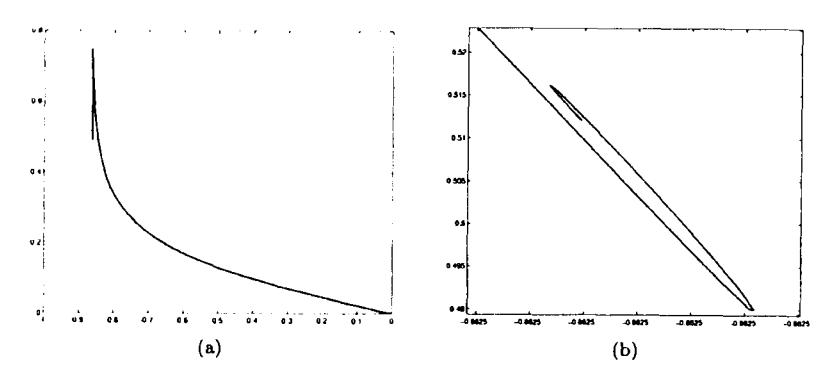
Figure 1: The relation between \(\gamma\) (vertical axis) and c (horizontal axis). Picture (b) magnifies a part of the plot (a). It contains the center of the spiral.
Somehow, near the edge of the IV-characteristic, we have a spiral shaped curve. Previously, this kind of spiral in the IV-characteristic has been observed in a single long Josephson junction by Brown et al. [4]. Later on, it is shown in [10, 11] that such a spiral exists in the single Josephson junction if the dissipation due to surface resistance, i.e. adding a term \(\beta \phi_{xxt}^{1,2}\) in Eq. (1), is taken into account.
However, there is a difference between the spiral we have in this case and spiral in a single long Josephson junction. The spiral in the single long Josephson junction has its
center located at |c| = 1 which is the maksimum velocity possibly achieved by a fluxon. In our case here, the center is below the lowest Swihart velocity \(|c_{+}| = \sqrt{1+S}\) [3]. The first four turning points are given in Table 1. The plot of the solitons related to those turning points is given in Figure 2.
| γ | с |
|---|---|
| 0.7489735 | -0.8622143 |
| 0.4900705 | -0.8625241 |
| 0.5161983 | -0.8625433 |
| 0.5121004 | -0.8625403 |
Table 1: The first four turning points of the curve in the \(\gamma - c\) space.
Goldobin et al. [5] give a 'proof' which shows that the fluxon in the state [1|0] with J=1 cannot pass the lowest Swihart velocity \(|c_+|\). The result says that if \(|c_+|\) is reached, there is at least a fluxon in the second junction which then gives the [1|1] state.
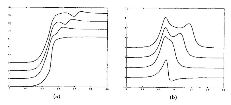
Figure 2: \(\phi^1\) (a) and \(\phi^2\) (b) as functions of \(\xi\) at the first four turning points. The lowest solution corresponds to the first turning point. The i-th solution is shifted (i-1) unit(s) in the vertical direction.
3 Unequal Junctions: J > 1
An interesting situation occurs if the two junctions forming the stack are not identical. We assume that only the critical currents of the two are unequal, which translates to the condition that J in Eq. (3) is not equal to 1.
Goldobin et al. [6] mention for the first time that there is a 'backbending' phenomenon in the IV-characteristic. With AUTO we can continue the backbending such that we get the full-branch of the IV-characteristic. The result is shown in Fig. 3.
Goldobin et al. [5] also show that the velocity \(|c_+|\) cannot be reached at this case.
In Fig. 4, two solutions for the same value of \(\gamma\) are plotted. In the first junction there is hardly any change, but in the second junction there is a big difference. On the left branch there is only a small 'image' in the second junction, which then if we follow the IV-characteristic, this image has grown to a large hump.
The stability of solutions on the right branch has been tested numerically in [11]. By taking the solution as calculated with AUTO and using this as initial solution to the PDE-solver [12], we conclude that all solutions on the right branch are unstable. All solutions at
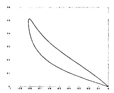
Figure 3: The IV-characteristic for J > 1.
the left branch up to the point where \(d\gamma/dc = 0\) are stable. Solutions on the right branch are in the domain of attraction of the solution for the same value of \(\gamma\) on the left branch.
The instability of the solution can be seen clearer when we follow the right branch in the direction of decreasing \(\gamma\). In the limit \(\gamma\) tends to 0, there is a fluxon-antifluxon pair in junction 2 or the stack is in [1|1,-1] [5]. Because the fluxon and antifluxon are attracting each other, if we apply a bias current, they will collide and a new different state is formed. This is the physical argument to show that this state is unstable.
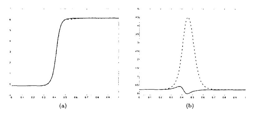
Figure 4: Comparison of two solutions to (3) for J=1.5 and \(\gamma=0.17\) on the left and right branch.
4 Unequal Junctions: J < 1
A somewhat different behavior happens when we look at case the J < 1. While in the case \(J \ge 1\), the velocity is bounded by \(c_+\), \(|c| \le |c_+|\), in the case J < 1 we have that |c| can exceed the value \(|c_+|\). When fluxons move with velocities above the lowest Swihart velocity, Cherenkov radiation takes place.
Cherenkov radiation is the emission of waves behind the moving fluxon. Behind the fluxon we will find an oscillating tail which is the emitted waves. E. Goldobin et al. [6, 7] observe Cherenkov radiation happening in the [1]0] state numerically and experimentally.
The IV-characteristic of the state is given in Fig. 5. Unfortunately, the IV-characteristic stops at \(c_{+}\) because our equation becomes singular at that value and AUTO cannot con-
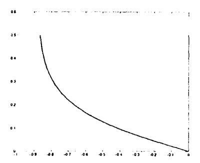
Figure 5: The IV-characteristic for J < 1.
tinue the calculation through the singularity. Therefore, all solutions that lie in this IV-characteristic do not have such emitted wave behind the fluxon as we see in Fig. 6.
If we keep increasing the applied bias current, the velocity of the fluxon increases up to the maximum velocity \(|u_{max}^{[1|0]}|\). This maximum velocity is a function of J, S, \(\alpha\) [6]. By now, the analytic form of the maximum velocity for this state is still unknown.
Another branch is found when we use one solution on the left branch of the IV-characteristic for J>1 as the initial solution of AUTO. Using this initial condition, then we decrease the parameter J up to J=0.5. In fact, we get a backbending curve for the IV-characteristic of the case J<1. The curve is given in Fig. 7. If for J>1, we see hardly any changes when comparing solutions in the first junction, while something different happens in the second junction (Fig. 4), for the case we have the opposite result. In junction 2 we almost have seen nothing, while there is a difference in the solutions in the first junction. In Fig. 8 we compare two solutions on the left and right branch for the same value of \(\gamma\).
A further analysis is needed to see the stability of solutions lying on this branch. We conjecture that all the solutions are unstable. The same argument might be used as in the case J>1 before. Numerical simulation confirms as well that the solutions go to the corresponding solutions at the other branch. We have done that also using PDE-solver where we use a solution resulted by AUTO as the initial solution of the PDE-solver.
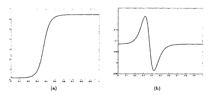
Figure 6: Solution to (3) for J = 0.5 and \(\gamma = 0.17\).
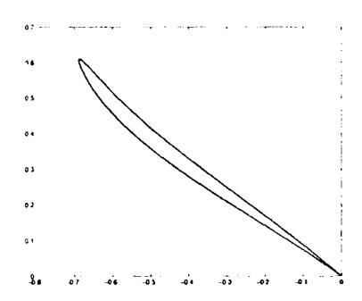
Figure 7: Another branch for the IV-characteristic of J < 1.
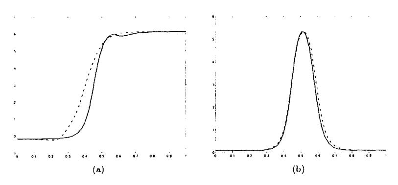
Figure 8: Comparison of two solutions to (3) for J=0.5 and \(\gamma=0.17\) on the left and right branch.
5 Conclusion
We have given several calculations showing that stacked-Josephson junctions have very rich behavior. Just with [1|0] state and changing J, we already have qualitatively different IV-characteristics, while there are many more states that can exist in the junctions.
How the IV-characteristics corresponding to the state [n|m] change when J passes through 1 needs to be investigated further. Also the stability of the various patterns needs to be determined.
Goldobin et al. [6] state that for the [1|0] state not only the condition J < 1 leads to \(|c| > |c_+|\), but also the asymmetry of the applied bias current of the two-fold stack, i.e. when we have \(\gamma^1 > \gamma^2\). Therefore, it might be interesting to consider also in the near future the possibility of having branches of the system under condition \(\gamma^1 \neq \gamma^2\).