

1. INTRODUCTION
In the last two decades, one has witnessed dramatic advances in photonic technology and its applications to modern communication and information processing, superseding to a large extent, the once dominant role of conventional microelectronics technology. The rapidly raising demand on communication speed and capacity has further pointed to the need of all optical technology for the realization of communication system operating beyond 10 Gbps for each carrier channel. An answer to this challenge is the development of optically controlled photonic devices or integrated optics. Such devices must operate on the basis of nonlinear optical effect such as the Intensity Dependence Refractive Index (IDRI) effect, described by the expression \(n = n_0 + n_2 I\) for the total refractive index n, where \(n_0\) and \(n_2\) are the linear and nonlinear refractive indices respectively and I is the light intensity.
One of the most important classes of optical devices is characterized by optical periodic structure consisting of two alternating dielectric media as illustrated in Fig.1. This basic periodic system can serve as a grating or waveguide system depending on the direction of light propagation. When light is illuminated in the x or y-direction, the system functions as a multilayer waveguide, and it functions as a grating when illuminated in the z-direction.
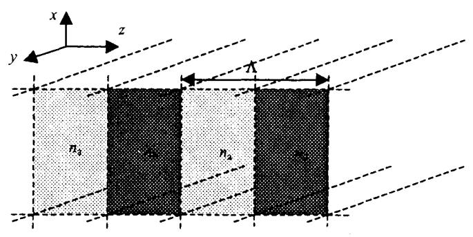
Fig.1. Optical periodic structure consisting of two alternating dielectric media of refractive indices \(n_a\) and \(n_b\) with periodicity \(\Lambda\).
An important feature of linear grating system is the presence of frequency bandgap, meaning that light with certain frequency lying in the band-gap cannot propagate through the system. The existence of a band-gap offers many useful applications of grating-assisted optical devices. A simple example is the optical filter as illustrated in Fig. (2a). Another example is the Add-drop channel device made by asymmetric graring coupler as illustrated in Fig. (2b), []. A component (2,) of the light having three different wavelengths (1"t,1r,23) will be reflected by the grating, coupled to the waveguide and transmitted out through the drop channel. Likewise a light with another wavelength (,to ) can be added through the add-channel and henceforth coupled to the grating resulting in an outgoing light consisting ofone different component (l.r,S.r.l.o) in the output channel.
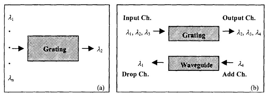
Fig.2. Optical devices (a) Filter (b) Add-drop Channel
The working principles of grating illustrated in fig. 2 can be operated in the passive or active mode. The incorporation of nonlinearity element such as IDRI effect in the device will allow it to function as an active device, with the light intensity playing as a control parameter. In this paper we shall stress our discussion on grating structure with optical Kerr media exhibitine IDRI cffect.
2. GENERAL FORMULATION
We start our discussion about the nonlinear optical periodic systems by considering the following one-dimensional Helmholtz equation:
\[\frac{\partial^2 E}{\partial z^2} + \beta_0^2 n^2 (z) E = 0 \tag{1}\] where po = aolc is the free space wave number. The total refractive index n is define as follows. Assuming ns(r)r2Q) .. ,l(t), *e shall write:
\[n(z) = n_0(z) + n_2(z)|E|^2. (2)\]
The periodic variation of the linear and nonlinear refractive indices along z-dircction are expanded in the following Fourier series:
\[n_{0,2}(z) = \overline{n}_{0,2} + \sum_{m \in Z \neq 0} \Delta \widetilde{n}_{0,2}^{(m)} \exp(imGz).\] (3)
Where G=2rl/t, which satisfies the Bragg condition G=2f0, n' is the average of refractive indices and At('') the m-th Fourier component of refractive index contrast. Here, we assume that the electric field E(z) can also be written in terms of Fourier series:
\[E = \sum_{m \in \mathbb{Z}} E^{(2m+1)} \exp(i\beta^{(2m+1)}z) + c.c\] (4)
where p(2''+t) =(Z^*t)p is the propagation constant of the (22+l)-th mode of the conesponding field E(2'*l), which satisfies the SVEA with respcct to z and t, and implies that the corresponding first order derivative 0Eldz is regarded as small but finite quantity, e. We assume further, as in ref. [2], the existencc of dominant forward and backward waves amplitudes E(l) sn6 p(-t) at the wave numbcr p. Substituting equarion (3) and (4) into equation (l) and denoting E(l) Uy,l anO E(-l) by B, we arrive at the following approximate coupled equations of the dominant fields:
\[i\frac{\partial A}{\partial z} + \delta_{1}A + \delta_{2} \left[ |A|^{2} + 2|B|^{2} \right] A + \delta_{3}B + \delta_{4} \left[ 2|A|^{2} + |B|^{2} \right] B + \delta_{4}A^{2}\overline{B} + \delta_{5}\overline{A}B^{2} = 0 , (5a)\]
\[-i\frac{\partial B}{\partial z} + \delta_1 B + \delta_2 \left[ B \right]^2 + 2|A|^2 B + \delta_3 A + \delta_4 \left[ 2|B|^2 + |A|^2 \right] A + \delta_4 B^2 \overline{A} + \delta_5 \overline{B} A^2 = 0 , (5b)\] where the coefficients d,'s are given as follows:
\[\delta_1 = \left(\beta^2 - \beta_0^2 \overline{n}_0^2\right)/2, \text{ detuning parameter,}\] (6a)
\[\delta_2 \propto \overline{n}_2\]. (6b)
\[\delta_3 \propto \left( \Delta \widetilde{n}_0^{(1)} + \sum_{m \neq 0, 1} \frac{\Delta \widetilde{n}_0^{(-m)} \Delta \widetilde{n}_0^{(m+1)}}{(2m+1)^2 - 1} \right), \tag{6c}\]
\[\delta_4 \propto \Delta \widetilde{n}_2^{(i)},\] (6d)
\[\delta_5 \propto \Delta \widetilde{n}_2^{(2)}\]. (6e)
As mentioned in the introduction, the existence of band gap is generally expected in linear grating. Due to its relevance to the ensuing discussion, this linear band gap will be briefly described and parameterizcd. To this end, let us consider the linear part of equation (5):
\[i\frac{\partial A}{\partial z} + \delta_1 A + \delta_3 B = 0 , \qquad (7a)\]
\[-i\frac{\partial B}{\partial z} + \delta_1 B + \delta_3 A = 0 . \tag{7b}\]
Taking the plane wave solutions for A and B as given by:
\[\begin{pmatrix} A \\ B \end{pmatrix} = \begin{pmatrix} A_0 \\ B_0 \end{pmatrix} e^{i\kappa z} \tag{8}\]
one is readily led to the following expression for \(\kappa\):
\[\kappa = \pm \sqrt{\delta_1^2 - \delta_3^2} \ . \tag{9}\]
Clearly, the linear band gap is characterized by the parameters \(\delta_1\) and \(\delta_3\) with \(\delta_1^2 < \delta_3^2\).
It is also straightforward to prove that the coupled equations (5) incorporate the conservation law:
\[|A|^2 - |B|^2 = C (10)\] where C is a constant. The case of C = 0 or zero energy flow condition is the focus of our study. This condition implies that A and B should be written as follows:
\[A(z) = f(z)\exp(i\phi(z)), \tag{11a}\]
\[B(z) = f(z)\exp(-i\phi(z)), \tag{11b}\] where the amplitude function f(z) and phase function \(\phi(z)\) are real functions. Substituting equation (11) into equations (5) will lead us to the following coupled equations:
\[\frac{\partial \phi}{\partial z} = \delta_1 + 3\delta_2 f^2 + \delta_3 \cos(2\phi) + 4\delta_4 f^2 \cos(2\phi) + \delta_5 f^2 \cos(4\phi), \tag{12a}\]
\[\frac{\partial f}{\partial z} = \delta_3 f \sin(2\phi) + 2\delta_4 f^3 \sin(2\phi) + \delta_5 f^2 \sin(4\phi). \tag{12b}\]
The corresponding Lagrangian for these equations is given by:
\[L = f^2 \frac{\partial \phi}{\partial z} - \delta_1 f^2 - \frac{3}{2} \delta_2 f^4 - \delta_3 f^2 \cos(2\phi) - 2\delta_4 f^4 \cos(2\phi) - \frac{1}{2} \delta_5 f^4 \cos(4\phi).\] (13)
Using the standard Legendre transformation we found the corresponding Hamiltonian as:
\[H(f^2, \phi) = \delta_1 f^2 + \frac{3}{2} \delta_2 f^4 + \delta_3 f^2 \cos(2\phi) + 2\delta_4 f^4 \cos(2\phi) + \frac{1}{2} \delta_5 f^4 \cos(4\phi), (14)\]
satisfying the canonical equations:
\[\frac{\partial \phi}{\partial z} = \frac{\partial H}{\partial f^2}, \qquad \frac{\partial f^2}{\partial z} = -\frac{\partial H}{\partial \phi}.\] (15)
It is readily proved that Hamiltonian (14) is also a conserved quantity i.e dH/dz = 0 and hence \(H(f^2, \phi) = h\), where h is a real constant. For a certain h and using equation (14), we can eliminate f(z) from equation (12a) and obtained a first order differential equation of \(\phi(z)\) as follows:
\[\frac{\partial \phi}{\partial z} = \pm \frac{1}{2} \sqrt{\left(2\delta_3^2 + 8h\delta_5\right) \cos(4\phi) + \left(8\delta_1\delta_3 + 32h\delta_4\right) \cos(2\phi) + 4\delta_1^2 + 2\delta_3^2 + 24h\delta_2}\] (16)
We can therefore find the solutions of coupled equations (12) simply by solving equation (16), and determine f(z) from equation (14).
The characteristics of the solution can be best elucidated by first identifying all the fixed points \((\bar{f}^2, \bar{\phi})\) of the Hamiltonian given by equation (14) according to the equations [3]:
\[\frac{\partial H}{\partial f^2} = P(f^2, \phi)_{(\bar{f}^2, \bar{\phi})} = 0, \qquad \frac{\partial H}{\partial \phi} = Q(f^2, \phi)_{(\bar{f}^2, \bar{\phi})} = 0. \tag{17}\]
To each fixed points determined by equations (17) and specified by certain \(\bar{f}^2\) and \(\bar{\phi}\), one obtains the corresponding values of h from equation (14). There are four distinct fixed points \((\bar{f}_i^2, \bar{\phi}_i)\), i=1, 2, 3, 4, corresponding to four different values of h listed below:
\[h_1 = 0, (18a)\]
\[h_2 = -\frac{(\delta_1 + \delta_3)^2}{2(3\delta_2 + 4\delta_4 + \delta_5)},\] (18b)
\[h_3 = -\frac{(\delta_3 - \delta_1)^2}{2(3\delta_2 - 4\delta_4 - \delta_5)},\] (18c)
\[h_4 = \frac{2\delta_1^2 \delta_5 + 3\delta_2 \delta_3^2 - 4\delta_1 \delta_3 \delta_4 - \delta_3^2 \delta_5}{8\delta_4^2 - 12\delta_2 \delta_5 + 4\delta_5^2}.\] (18d)
It should be noted that a physical solution must satisfy the condition \(\tilde{f}_i^2 \ge 0\), i = 1, 2, 3, 4.
The characteristic variations of P and Q with respect to \(f^2\) and \(\phi\) in the close vicinity of a certain fixed point can be found by solving the following equation:
\[\begin{pmatrix} \frac{\partial f^2}{\partial z} \\ \frac{\partial \phi}{\partial z} \end{pmatrix} = \begin{pmatrix} \frac{\partial P}{\partial f^2} & \frac{\partial P}{\partial \phi} \\ \frac{\partial Q}{\partial f^2} & \frac{\partial Q}{\partial \phi} \end{pmatrix} \begin{pmatrix} f^2 \\ \phi \end{pmatrix},\] (19)
obtained by Taylor expanding P and Q around the fixed points. The solutions of these equations for each i will be of the form \(\exp(\lambda_i z)\), where \(\lambda_i\) is the eigenvalue of the corresponding operator:
\[A_{i} = \begin{pmatrix} \frac{\partial P}{\partial f^{2}} & \frac{\partial P}{\partial \phi} \\ \frac{\partial Q}{\partial f^{2}} & \frac{\partial Q}{\partial \phi} \end{pmatrix}, \tag{20}\]
evaluated at the corresponding fixed points \((\bar{f}_i^2, \bar{\phi}_i)\). A localized physical solution can only be found in concurrence with the existence of a saddle points specified by the condition \(\lambda_i^2 \ge 0\).
3. DEEP NONLINEAR BRAGG GRATING
A deep nonlinear Bragg grating is a Bragg grating system in which its refractive index contrast is comparable to their average, \(\Delta n/\bar{n} \approx \eta\), where \(\eta\) is a small but finite quantity. The dominant fields are governed by equations (5) with the coefficients \(\delta_i\)'s are given by equations (6). The influences of Fourier component of \(n_0\) corresponding to the non-dominant modes are incorporated in the coefficient \(\delta_3\) as indicated by the presence of second term in equation (6c). In this model, the coefficient \(\delta_2\) may have the same order with \(\delta_4\) and \(\delta_5\) by design. The coefficients \(\delta_3\), \(\delta_4\) and \(\delta_5\) are generally complex quantities but they are chosen to be real quantities in this study. Vanishing \(\delta_4\) and \(\delta_5\) will lead us to the equations of conventional shallow nonlinear Bragg grating with uniform nonlinearity [4].
In principle, we can study the quantitative behavior of the solutions of equations (12) by analyzing the phase portrait of H given by equation (14) in a Cartesian coordinates defined by the following transformation:
\[f^2 = x^2 + y^2\], \(\cos^2(\phi) = x^2/(x^2 + y^2)\), \(\sin^2(\phi) = y^2/(x^2 + y^2)\). (21)
Accordingly, Hamiltonian can be expressed in terms of Cartesian coordinate as follows:
\[H(x,y) = \delta_1(x^2 + y^2) + \frac{3}{2}\delta_2(x^2 + y^2)^2 + \delta_3(x^2 - y^2) + 2\delta_4(x^4 - y^4) + \frac{1}{2}\delta_5(x^4 - 6x^2y^2 + y^4). \tag{22}\]
In the case of h=\, th€ existence of localized solution with double hump gap soliton solutions ( di . rrz ) has already been known for some time [3]. It was pointed out in ref. [3] however that the double hump gap solitons are allowed only in the case of negative detuning (dr <0). In our study, we found that even for the case of positive detuning (dr >0), the double hump gap solitons also exist as illustrated in fig.(3a). We note that those two cases are of different shapes and intensities, and occurring at diffcrcnt phase (0)
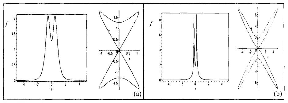
Fig.3. Doubte hump solitons with coefficient set 62 = l, 6t = 3, da = 9.75, ds = 2.5 for (a) positive detuning dr = I (b) negative detuning dt = - I
For the other non-vanishing Hamiltonians thr,ht,fta), equations (5) does not admits any localized solutions with vanishing tail. Nevertheless, in-gap and out-gap localized solutions with background known as dark and anti-dark soliton are allowed. Remarkably, contrary to the shallow grating case, due to the presence of da and d5 terms in the deep nonlinear Bragg grating has allowed us to find the in-gap dark and antidark solitons in addition to the out-gap dark and anti-dark solitons.
Instead of investigating the case of h = hz,l, which has been work out previously [5], we choose to focus on the cases for h=ho.lnfig.4 we give two illustrations of outgap dark soliton anti-dark soliton and the corresponding phase portrait for h=ha and ds = 0 (equal thickness of altemating layer). It is clear from both figures that for a set of coefficients, dark and anti-dark solitons exists in a complementary trajectory sections of an ellipse, denoted by the solid bold lines are the trajectories of corresponding solutions. These solid bold lines connecting two interscction points which are actually the unstable points. The circular arcs in between correspond to the constant solutions. In addition to the out-gap soliton solutions, the in-gap dark soliton is also exist as illustrated in fig.5 along with its conesponding phase portrait. For the case of dr = O, we only found the dark soliton solutions since thc only trajectorics connecting the two unstable points are inside the circle.
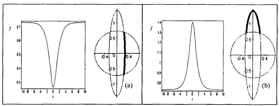
Fig.4. Out-gap (a) dark and (b) anti-dark soliton with coefficients set \(\delta_1 = 1, \delta_2 = -1, \delta_3 = 0.75, \delta_4 = -0.7, \delta_5 = 0\)
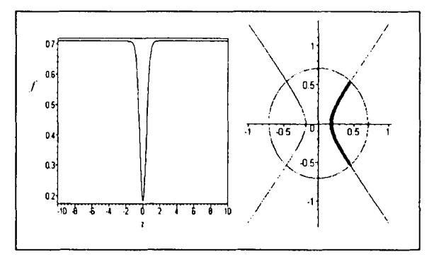
Fig.5. In-gap dark soliton with coefficients set \(\delta_1 = 1\), \(\delta_2 = -1\), \(\delta_3 = 3\), \(\delta_4 = -3\), \(\delta_5 = 0\)
In the case \(\delta_5 \neq 0\), the circles in the phase portraits presented in fig.4 and 5 are distorted into ellipses including in addition to the in-gap dark soliton, the anti-dark soliton as well. This situation is illustrated in fig.6. These in-gap dark and anti-dark solitons are unique for deep nonlinear Bragg grating, but they have never been reported before.
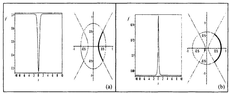
Fig. 6. Soliton with coefficients set \(\delta_1 = 1\), \(\delta_2 = -1\), \(\delta_3 = 3\), \(\delta_4 = -3\) (a) \(\delta_5 = -1\) for dark soliton (b) \(\delta_5 = 1\) for anti-dark soliton.
Complete classifications and detailed explicit expressions of dark and anti-dark solitons in deep nonlinear Bragg grating can be found in ref.[6].
4. SHALLOW NONLINEAR BRAGG GRATING WITH NONLINEAR MODULATION
In contrasto the case of deep nonlinear Bragg grating, where we assumed that the refractive indices contrast are comparablc to their average, in the casc of shallow nonlinear Bragg grating with nonlinear modulation, the ratio between these two quantities Molfro and Ln2fn, are both smaller than 7 in the deep grating. We can assume therefore that the electric field f(z) in this case can simply written as follows:
\[E(z) = A(z)\exp(i\beta z) + B(z)\exp(-i\beta z)\] (20)
wherc ,4 and B are the forward and backward propagating field envelopcs rcspcctivcly, with p denoting the single mode wave number. Differing from the conventional shallow nonlinear Bragg grating, we consider here the system, which operates with optical wave having field intensity lOl2 large enough to enhance the IDRI effect, so that the nonlinear modulation effect becomes significant. In other words, we shall keep working with the equation (5) and retaining the da and 55 terms which where neglected in the conventional case [4].
Specializing to the single mode solution of equation (20), the d, coefficient given by equation (6c) reduces to d, cc Ais while the other coefficients remain unchanged. While this equation can be formally treated in thc same manner as the previous case, the solutions found are basically the same as those found in the conventional shallow nonlinear Bragg grating. The presence of da and 6, does affect the width and height of the localized solutions. A complctc and comprchcnsive discussion on this casc can bc found in ref. [7].
Although the equations for both deep nonlinear Bragg grating and shallow nonlinear Bragg grating with nonlinear modulation are the same, but, the order of thcir coefficients are differcnt, so, as a consequenc€s, not all solutions admitted in dcep nonlincar Bragg grating are valid for the shallow case.
5. CONCLUSIONS
The existence of in-gap dark and anti-dark solitons and double hump gap soliton solutiorrs in decp nonlinear Bragg grating has been demonstrated for the first time by using the phase plane analysis. These solutions are unique for decp nonlinear Bragg grating and cannot be found in a conventional shallow nonlinear Bragg grating, or the system with large IDRI enhancement.
6. ACKNOWLEDEMENT
H.A. would like to thank to the KNAW supporred EPAM-Project for giving him a chance to visit the University of Twente, The Netherlands. Also to the Lightrvave
Device Group (LDG) and Applied Analysis and Mathematical Physics (AAMP) Group, MESA+ Institute, University of Twente for hospitality during his visit.
7. REFERENCES
- 1. T. Erdogan, Opt. Comm. 157, 249 (1998)
- 2. T. Iizuka, C. M. de Sterke, Phys. Rev. E 61, 4491 (2000)
- 3. F. Verhulst, Nonlinear Differential Equations and Dynamical Systems, Springer-Verlag (1990)
- 4. C. M. de Sterke, J.E. Sipe, in Progress Optics, edited by E. Wolf (North-Holland, Amsterdam). 33, 203 (1994)
- 5. Y.S. Kivshar, N. Flytzanis, Phys. Rev A, 46(12), 7972 (1992)
- 6. H. Alatas, A.A. Iskandar, M.O. Tjia, T.P. Valkering, Submitted to J. Non. Lin. Opt. Phys. and Mater.
- 7. H. Alatas, A.A. Iskandar, M.O. Tjia, to be submitted to Kont. Fis. Ind.
fo a
Ir fu
va X i.e 0,