
1 Introduction
An observation at a certain spatial location and time may be commonly influenced by previous-time observations in that location and its neighboring locations. For example, the oil production of a certain well during this month can be affected by the production during the previous months at that same location and at the neighboring wells; the number of today's criminal actions in a city may be influenced by the number of criminal actions that happened during the previous days in that city and the nearest cities; or, then the number of vehicles at a certain intersection within a certain time range is influenced by the number of vehicles at that location and related intersections during the previous time ranges. These examples are the portrait of space-time analysis problems.
Also, we would like to be able to forecast the oil production of that particular well during the coming months; how many criminal actions will happen in the city; and how many vehicles can be found at that particular intersection during the next range times. Knowing these forecasts, people in charge may take the necessary actions. We can do forecasting after obtaining the appropriate model. One way of doing this is space-time modeling.
In this paper we proffer a new procedure for space-time modeling, especially for Generalized STAR (GSTAR) modeling. For this purpose, we modify the Pfeifer and Deutsch three stage-iterative procedure for space-time modeling
(see [1]), which consist of identification, parameter estimation and diagnostic checking. We improve model selection by checking the stationarity of possible models using the IAcM. The IACM has been studied for autoregressive models of time-series by Rahardjo in 2005 [2]. We will explain these processes briefly in Section 3. Before that, we will describe the GSTAR model and spatial weight matrices in Section 2. In Section 4, we employ real data of the monthly tea production in some plantations in West Java. Finally Section 5 contains remarks and conclusions.
2 Generalized STAR Model
The observation at site i and time t, \(Y_{i,t}\), which is a realization of a stochastic process, follows the GSTAR model if it can be declared as a linier combination of past observations for both time and spatial indices. A \((N\times 1)\)-dimensional centered process vector \(\mathbf{Y}_t = (Y_{1,t}, Y_{2,t}, ..., Y_{N,t})'\) follows the GSTAR(\(p; \lambda_1, \lambda_2, ..., \lambda_n\)) model if \(\mathbf{Y}_t\) can be presented as,
\[\mathbf{Y}_{t} = \sum_{k=1}^{p} \sum_{\ell=0}^{\lambda_{k}} \mathbf{\Phi}_{k\ell} \mathbf{W}^{(\ell)} \mathbf{Y}_{t-k} + \mathbf{e}_{t}\] (1)
with k is time autoregressive order \((k=1,\,2,\,...,\,p),\,\ell\) is spatial autoregressive order \((\ell=0,\,1,...,\,\lambda_k)\), and \(\mathbf{e}_t\) is \((N\times 1)\)-dimensional vector of errors that assumed have i.i.d normal distribution. The \(\mathbf{W}^{(\ell)}\) is \(\ell\)-th order weight matrix which the main diagonal is zero and the sum of each row is one, and \(\mathbf{\Phi}_{k\ell}\) is \((N\times N)\) diagonal matrix which presents autoregressive parameter of k-th time order and \(\ell\)-th spatial order for each location \(i=1,\,2,\,...,\,N\). We write \(\mathbf{\Phi}_{k\ell}=\mathrm{diag}\left(\phi_{k\ell}^{(1)},\phi_{k\ell}^{(2)},...,\phi_{k\ell}^{(N)}\right)\).
Figure 1 Spatial order/lag in two dimensional radius system. Sites in same 'category of distance' are in the same spatial order. The category of distance is classified by a fixed radius value \(d_0\).
The \(\ell\)-th spatial order shows the ordered neighbors of a number of spatial locations, while spatial weight \(w_{ij}^{(\ell)}\) shows the influence of location j on location i in spatial lag \(\ell\)-th. The locations which are closer to the reference location \((s_0)\) will have a smaller spatial lag, which is distinguished by fixed distance \(d_0\) (Figure 1). Since the configuration in each spatial lag order is distinct, different spatial lags may give different weight matrices.
2.1 Spatial Weights
There are three types of spatial weight: binary, uniform, and non-uniform. Binary weight matrix has values 0 and 1 in off-diagonal entries; uniform weight is determined by the number of sites surrounding a certain site in \(\ell\)-th spatial order; and non-uniform weight gives unequal weight for different sites. The element of the uniform weight matrix is formulated as,
\[w_{ij}^{(\ell)} = \begin{cases} \frac{1}{n_i^{(\ell)}} & \text{, } j \text{ is neighbor of } i \text{ in } \ell\text{-th order} \\ 0 & \text{, others} \end{cases}\]
\(n_i^{(\ell)}\) is the number of neighbor locations with site-i in \(\ell\)-th order.
The non-uniform weight may become uniform weight when some conditions are met. One method in building non-uniform weight is based on inverse distance, which is used by Borovkova in 2008 [3]. The weight matrix of spatial lag k is based on the inverse weights \(\frac{1}{1+d_{ij}}\) for sites i and j whose Euclidean distance \(d_{ij}\) lies within a fixed distance range, and otherwise is weight zero.
2.2 Stationarity
GSTAR models are invertible since the vector of observations \(\mathbf{Y}_t\) could be expressed as a weighted linear combination of past observations with weights that converge to zero. In order for a GSTAR model to represent a stationary process, one in which the covariance structure of \(\mathbf{Y}_t\) does not change with time, certain conditions should be met. We obtain the stationary conditions of the first and second order of GSTAR models using its IAcM by the following propositions.
Proposition 1 Suppose that \((N \times N)\)-dimensional matrix \(\mathbf{A} = \Phi_{10} + \Phi_{11} \mathbf{W}\) and IAcM, \(\mathbf{M_1} = \mathbf{I}_N - \mathbf{A'A}\), is invers of autocovariance matrix whose elements are the parameters of GSTAR(1;1) process. If the determinants of all the leading principal submatrices of IAcM are positive, then GSTAR(1;1) model is stationary.
Proof. The IAcM is built from the sum square of errors from all past observations until the first observation. For \((N\times 1)\)-dimensional vector of observations, \(\mathbf{Y}_1 = (Y_{1,1}, Y_{2,1}, \dots, Y_{N,1})'\), we can write \(\mathbf{Y}_1'\mathbf{M}_1\mathbf{Y}_1 = \sum_{t=-\infty}^1 \mathbf{e}_t'\mathbf{e}_t\) which has positive and finite values. The \(\mathbf{M}_1\) is symmetric and since \(\mathbf{Y}_1'\mathbf{M}_1\mathbf{Y}_1 > 0\) then \(\mathbf{M}_1\) is positive definite matrix [4]. It implies the determinants of all leading principal submatrices of \(\mathbf{M}_1\) are positive. Furthermore, since \(\mathbf{M}_1\) and the covariance structure is do not change with the time, the GSTAR(1;1) process is stationary. Q.E.D.
The IAcM is a symmetric positive definite matrix. For GSTAR(1; \(\lambda_1\)) models with \(\lambda_1 \geq 0\), we may define \(\mathbf{A} = \sum_{\ell=0}^{\lambda_1} \mathbf{\Phi}_{1\ell} \mathbf{W}^{(\ell)}\), and the IAcM is,
\[\mathbf{M_1} = \mathbf{I}_N - \mathbf{A}'\mathbf{A} \tag{2}\]
Proposition 2 GSTAR(1; \(\lambda_1\)) models are stationary if the determinants of all the leading principal submatrices of \(M_1\) are positive.
Proof. Similar to Proposition 1, suppose \(\mathbf{Y}_1\) is a \((N \times 1)\)-dimensional vector of observations, \(\mathbf{Y}_1 = (Y_{1,1}, Y_{2,1}, ..., Y_{N,1})'\). The \(\mathbf{Y}_1'\mathbf{M}_1\mathbf{Y}_1\) is the collection of squared errors from all past observations until the first observation. This means that \(\mathbf{Y}_1'\mathbf{M}_1\mathbf{Y}_1\) always has positive value and is only equal to null if \(\mathbf{Y}_1\) is a null vector. We write,
\[\mathbf{Y}_1'(\mathbf{I} - \mathbf{A}'\mathbf{A})\mathbf{Y}_1 > 0\]
\(\|\mathbf{Y}_1\|^2 - \|\mathbf{A}\mathbf{Y}_1\|^2 > 0\)
\(\|\mathbf{A}\mathbf{Y}_1\|^2 < \|\mathbf{Y}_1\|^2\)
The absolute eigen value of A must be less than one, which means that the GSTAR(1; \(\lambda_1\)) process is stationary. Q.E.D.
The stationarity condition in Proposition 1 and 2 meets the stationarity condition that was formulated by Wei [5] for Vector AR models. Furthermore for GSTAR(2; \(\lambda_1\), \(\lambda_2\)) models, we define (\(N \times N\))-dimensional matrix
\[\mathbf{A}_k = \sum_{\ell=0}^{\lambda_k} \mathbf{\Phi}_{k\ell} \mathbf{W}^{(\ell)}\], \(k = 1, 2\) and the \((2N \times 2N)\)-dimensional IAcM is,
\[\mathbf{M}_{2} = \begin{pmatrix} \mathbf{I}_{N} - \mathbf{A}_{2}^{'} \mathbf{A}_{2} & -\mathbf{A}_{1}^{'} - \mathbf{A}_{2}^{'} \mathbf{A}_{1} \\ -\mathbf{A}_{1} - \mathbf{A}_{1}^{'} \mathbf{A}_{2} & \mathbf{I}_{N} - \mathbf{A}_{2}^{'} \mathbf{A}_{2} \end{pmatrix}\](3)
Proposition 3 GSTAR(2; \(\lambda_1\), \(\lambda_2\)) models are stationary if the determinants of all the leading principal submatrices of its IAcM are positive.
Proof. Using a similar procedure as with Proposition 2 and by letting \(\mathbf{Y}_2 = (Y_{1,1}, ..., Y_{N,1}, Y_{1,2}, ..., Y_{N,2})'\), we may consider Proposition 3 as proved. Q.E.D
These stationarity conditions can provide a significance contribution to the process of identifying possible GSTAR models.
3 Identification Process GSTAR Model
A GSTAR model is a generalization of a STAR model with respect to its parameters. In a STAR model, the parameters are assumed to be the same for every location, while a GSTAR model assumes that different locations have different parameter values. Although both have different assumptions concerning the parameters, they still have the same procedures in doing the identification process of space-time models.
3.1 Space Time ACF and PACF
The STACF and STPACF had been employed by Pfeifer and Deutsch [1] in identifying Space-Time Autoregressive Moving Average (STARMA) models. Since STARMA and GSTAR models have many things in common, STACF and STPACF may be applied in identifying GSTAR models. The STACF is obtained by standardizing the autocovariance function of lag time s for observations with lag spatial k-th and \(\ell\)-th, \(\gamma_{\ell k}(s)\). Autocovariance function in matrix notation is
\[\gamma_{\ell k}(s) = \frac{1}{N} E \left[ \left( \mathbf{W}^{(\ell)} \mathbf{Y}_{s} \right)' \left( \mathbf{W}^{(k)} \mathbf{Y}_{t+s} \right) \right]\] (4)
Since equation (4) is a scalar then we write
\[\gamma_{\ell k}\left(s\right) = \frac{1}{N} tr\left\{\mathbf{W}^{(\ell)} \mathbf{W}^{(k)} E\left[\mathbf{Y}_{t}' \mathbf{Y}_{t+s}\right]\right\} = \frac{1}{N} tr\left\{\mathbf{W}^{(\ell)} \mathbf{W}^{(k)} \Gamma\left(s\right)\right\}\] (5)
The estimator for \(\Gamma(s)\) is \(\hat{\Gamma}(s) = \sum_{t=1}^{T-s} \frac{\mathbf{Y}_t \mathbf{Y}_{t-s}}{T-s}\) and by substituting it to (5) then estimated covariance, \(\hat{\gamma}_{\mathbb{R}}(s)\) holds. Furthermore the STACF, which is defined as,
\[\rho_{\ell k}(s) = \frac{\gamma_{\ell k}(s)}{\left[\gamma_{\ell \ell}(0)\gamma_{k k}(0)\right]^{1/2}}\]
can be estimated by using the sample covariance,
\[\hat{\rho}_{\ell k}(s) = \frac{\hat{\gamma}_{\ell k}(s)}{\left[\hat{\gamma}_{\ell \ell}(0)\hat{\gamma}_{k k}(0)\right]^{1/2}} = \frac{\sum_{i=1}^{N} \sum_{i=1}^{T-s} L^{(\ell)} Y_{i,t} L^{(k)} Y_{i,t+s}}{\left[\sum_{i=1}^{N} \sum_{t=1}^{T} \left(L^{(\ell)} Y_{i,t}\right)^{2} \sum_{i=1}^{N} \sum_{t=1}^{T} \left(L^{(k)} Y_{i,t}\right)^{2}\right]^{1/2}}\](6)
with \(\mathit{L}^{(\ell)}\) as the spatial lag operator of spatial order \(\,\ell\) -th, so that
\[L^{(\ell)}Y_{i,t} = \begin{cases} Y_{i,t}, & \ell = 0\\ \sum_{j=1}^{N} w_{ij}^{(\ell)} Y_{j,t}, & \ell = 1, 2, ..., \lambda_p \end{cases}\] the STPACF for spatial order \(\lambda\) is the last coefficient of \(\phi_{h\ell}\) (\(\ell=0,1,\ldots,\lambda\) and \(h=1,2,\ldots\)) in space-time Yule Walker equation as defined in [1].
| \[\begin{bmatrix} \gamma_{00} \left( 1 \right) \\ \gamma_{10} \left( 1 \right) \\ \vdots \\ \gamma_{n-1} \left( 1 \right) \end{bmatrix}\] | \[\begin{bmatrix} \gamma_{00} (0) \\ \gamma_{10} (0) \\ \vdots \\ \gamma_{10} (0) \end{bmatrix}\] | \(\gamma_{01}(0) \cdots \\ \gamma_{11}(0) \cdots \\ \vdots \\ \vdots\) | \[\gamma_{0\lambda}(0) \\ \gamma_{1\lambda}(0) \\ \vdots \\ \vdots\] | \[\begin{vmatrix} \gamma_{00} \left(-1\right) \\ \gamma_{10} \left(-1\right) \\ \vdots \\ \cdots \left(-1\right) \end{vmatrix}\] | \(\gamma_{01} \left(-1\right)\) \(\gamma_{11} \left(-1\right)\) \(\vdots\) | \[\begin{array}{ccc} \cdots & \gamma_{0\lambda} \left(-1\right) \\ \cdots & \gamma_{1\lambda} \left(-1\right) \\ & \vdots \\ \cdots & \gamma_{\lambda\lambda} \left(-1\right) \end{array}\] | (1-h) | \(\left[\begin{array}{c} \phi_{10} \ \phi_{11} \ \vdots \ \phi_{0} \end{array}\right]\) | (7) |
|---|---|---|---|---|---|---|---|---|---|
| \[\begin{vmatrix} \frac{\gamma_{\lambda 0}(1)}{\gamma_{00}(2)} \\ \gamma_{10}(2) \\ \vdots \end{vmatrix}\] | \(\gamma_{\lambda 0}(0)\) | γλλ (0) | \(\gamma_{\lambda 0}(-1)\) | ··· γλλ (-1) | (2, 1) | \(\begin{array}{c} \phi_{1\lambda} \ \phi_{20} \ \phi_{21} \ \vdots \end{array}\) | (,) | ||
| \[\begin{vmatrix} \vdots \\ \frac{\gamma_{\lambda 0}(2)}{\vdots} \end{vmatrix} =\] | : | (1) | : | : | (0) | ÷ | (2-h) | \(\frac{\phi_{2\lambda}}{\vdots}\) | |
| \(\begin{bmatrix} \overline{\gamma_{00}\left(h\right)} \ \gamma_{10}\left(h\right) \ \vdots \ \gamma_{\lambda0}\left(h\right) \end{bmatrix}\) | (h-1) | (h-2) | (0) | \(\begin{bmatrix} \boldsymbol{\phi}_{p0} \ \boldsymbol{\phi}_{p1} \ \vdots \ \boldsymbol{\phi}_{h\lambda} \end{bmatrix}\) |
Space time model selection may be obtained by observing autocorrelation behavior among time lags and spatial lags which are represented by the cut off and tail off pattern of the STACF and STPACF.
3.2 IAcM as a Part of GSTAR Modeling
In this paper we propose a new procedure for GSTAR modeling by involving stationarity investigation through the IAcM characteristics as presented in Proposition 1 to 3. This stage is executed after identifying the model through the STACF and STPACF, and estimating the parameters. We see it as a first stage of model validation in addition to checking the mean square of residuals as the second stage. The residuals are obtained from the differences between real and estimated observations. The model with the minimum mean square of residuals will be recommended as the fitting model. The procedure of GSTAR modeling is shown in the following flow chart (Figure 2).
This procedure combines and advances the three-stage iterative procedure for space-time modeling of Pfeifer & Deutsch [1] and time-series modeling of Box & Jenkins [6]. The new aspect of this procedure is the process stationarity check with the IAcM *).
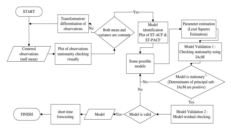
Figure 2 The new procedure of space time autoregressive modeling.
4 Case Study
For our case study we used the data of the monthly tea production of six plantation sites (N=6) in West Java, Indonesia (Purbasari, Santosa, Sedep, Papandayan, Cisaruni, and Dayeuh Manggung), from January 1992 to December 2010 (T=228). We executed space-time modeling by using Matlab and started by centering the processes in order to obtain the null mean of the processes. The coordinates of the observed plantations and the distances between them are displayed in a symmetric (\(N\times N\))-dimensional matrix of which the main diagonal is null (see Figure 3).
From Figure 3 we can draft the numbers of spatial lag order and its members, and also the weight matrices for each spatial lag. We can build the range of spatial lag based on the fixed radius system in Figure 1 with a fixed \(d_0\) of 0.4 km. The interval distance (0, 0.4] is categorized as spatial lag 1, (0.4, 0.8] as spatial lag 2, and so on until (0.4(-1), 0.4] as spatial lag \(\ell\). For this case we got four spatial lags for eachweight matrix (uniform, euclidean-uniform and binary). The appropriate weight matrices for the first and second spatial lag are shown in Table 1.
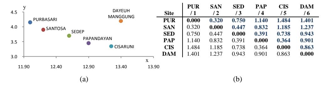
Figure 3 (a) The coordinate of six observed plantations, and (b) the distances (in kilometre, km). PUR is Purbasari, SAN is Santosa, SED is Sedep, PAP is Papandayan, CIA is Cisaruni, and DAM is Dayeuh Manggung.
Table 1 The weight matrices for spatial lag \(\ell\)-th, \(\ell = 1,2,3,4\). For \(\ell = 0\), the weight matrix \(\mathbf{W}^{(0)} = \mathbf{I}_N\). The sum of each row must be equal to one with a null main diagonal.
| Uniform | Euclidean - Uniform | Biner | |
|---|---|---|---|
| \(\mathbf{W}^{(1)}\) | \[\begin{pmatrix} 0 & 1 & 0 & 0 & 0 & 0 \\ 1 & 0 & 0 & 0 & 0 & 0 \\ 0 & 0 & 0 & 1 & 0 & 0 \\ 0 & 0 & 0.5 & 0 & 0.5 & 0 \\ 0 & 0 & 0 & 1 & 0 & 0 \\ 0 & 0 & 0 & 0 & 1 & 0 \end{pmatrix}\] | \[\begin{pmatrix} 0 & 1 & 0 & 0 & 0 & 0 \\ 1 & 0 & 0 & 0 & 0 & 0 \\ 0 & 0 & 0 & 1 & 0 & 0 \\ 0 & 0 & 0.495 & 0 & 0.505 & 0 \\ 0 & 0 & 0 & 1 & 0 & 0 \\ 0 & 0 & 0 & 0 & 1 & 0 \end{pmatrix}\] | \[\begin{pmatrix} 0 & 1 & 0 & 0 & 0 & 0 \\ 1 & 0 & 0 & 0 & 0 & 0 \\ 0 & 0 & 0 & 1 & 0 & 0 \\ 0 & 0 & 1 & 0 & 0 & 0 \\ 0 & 0 & 0 & 1 & 0 & 0 \\ 0 & 0 & 0 & 0 & 1 & 0 \end{pmatrix}\] |
| \(\mathbf{W}^{(2)}\) | \[\begin{pmatrix} 0 & 0 & 1 & 0 & 0 & 0 \\ 0 & 0 & 1 & 0 & 0 & 0 \\ 1/3 & 1/3 & 0 & 0 & 1/3 & 0 \\ 0 & 1 & 0 & 0 & 0 & 0 \\ 0 & 0 & 1 & 0 & 0 & 0 \\ 0 & 0 & 0 & 1 & 0 & 0 \end{pmatrix}\] | \[\begin{pmatrix} 0 & 0 & 1 & 0 & 0 & 0 \\ 0 & 0 & 1 & 0 & 0 & 0 \\ 0.311 & 0.376 & 0 & 0 & 0.313 & 0 \\ 0 & 1 & 0 & 0 & 0 & 0 \\ 0 & 0 & 1 & 0 & 0 & 0 \\ 0 & 0 & 0 & 1 & 0 & 0 \end{pmatrix}\] | \[\begin{pmatrix} 0 & 0 & 1 & 0 & 0 & 0 \\ 0 & 0 & 1 & 0 & 0 & 0 \\ 0 & 0 & 0 & 0 & 1 & 0 \\ 0 & 1 & 0 & 0 & 0 & 0 \\ 0 & 0 & 1 & 0 & 0 & 0 \\ 0 & 0 & 0 & 1 & 0 & 0 \end{pmatrix}\] |
| \(\mathbf{W}^{(3)}\) | \[\begin{pmatrix} 0 & 0 & 0 & 1 & 0 & 0 \\ 0 & 0 & 0 & 0.5 & 0.5 & 0 \\ 1 & 0 & 0 & 0 & 0 & 0 \\ 1/3 & 1/3 & 0 & 0 & 0 & 1/3 \\ 0 & 0.5 & 0 & 0 & 0 & 0.5 \\ 0 & 0 & 1/3 & 1/3 & 1/3 & 0 \end{pmatrix}\] | \[\begin{pmatrix} 0 & 0 & 0 & 1 & 0 & 0 \\ 0 & 0 & 0 & 0.544 & 0.456 & 0 \\ 1 & 0 & 0 & 0 & 0 & 0 \\ 0.304 & 0.355 & 0 & 0 & 0 & 0.342 \\ 0 & 0.460 & 0 & 0 & 0 & 0.540 \\ 0 & 0 & 0.326 & 0.334 & 0.340 & 0 \\ \end{pmatrix}\] | \[\text{[rumus tidak dapat ditampilkan dengan baik — lihat PDF asli]}\] |
| \(\mathbf{W}^{(4)}\) | \[\begin{pmatrix} 0 & 0 & 0 & 0 & 0.5 & 0.5 \\ 0 & 0 & 0 & 0 & 0 & 1 \\ 0 & 0 & 0 & 0 & 0 & 1 \\ 1 & 0 & 0 & 0 & 0 & 0 \\ 1 & 0 & 0 & 0 & 0 & 0 \\ 0.5 & 0.5 & 0 & 0 & 0 & 0 \end{pmatrix}\] | \[\text{[rumus tidak dapat ditampilkan dengan baik — lihat PDF asli]}\] | \[\begin{pmatrix} 0 & 0 & 0 & 0 & 0 & 1 \\ 0 & 0 & 0 & 0 & 0 & 1 \\ 0 & 0 & 0 & 0 & 0 & 1 \\ 1 & 0 & 0 & 0 & 0 & 0 \\ 1 & 0 & 0 & 0 & 0 & 0 \\ 0 & 1 & 0 & 0 & 0 & 0 \end{pmatrix}\] |
The appropriate weight of the matrices in Table 1 has similar values. This is acceptable because they have the same criterion for determining the spatial lag interval. This happens because there are only six observed sites, which should be categorized into four levels of spatial authority (\(\lambda_p = 4\)). Since there is subjective judgment involved in building the weight matrices, we should pay more attention to the rules, especially when the ratio between the number of locations and the number of spatial lags is close to 1:1. In these cases, it will be more difficult to obtain appropriate and obedient weight matrices.
The first stage in GSTAR modeling is to identify possible models by computing the STACF and STPACF values as in equation (6) and (7). These values are presented in Table 2.
| STA | |||||||||||
|---|---|---|---|---|---|---|---|---|---|---|---|
| STPACF | |||||||||||
| spatial lag time lag | 0 | 1 | 2 | 3 | 4 | spatial lag time lag | 0 | 1 | 2 | 3 | 4 |
| 1 | 0.4697 | 0.3102 | 0.3315 | 0.1989 | 0.3329 | 1 | 0.3578 | -0.0086 | 0.1975 | -0.0984 | 0.0634 |
| 2 | 0.1554 | 0.006 | 0.0105 | -0.0339 | 0.0401 | 2 | 0.0191 | -0.0385 | -0.2131 | 0.1136 | -0.0886 |
| 3 | 0.0699 | -0.0779 | -0.0912 | -0.1194 | -0.0532 | 3 | 0.1688 | 0.076 | -0.088 | -0.0345 | -0.0845 |
| 4 | -0.0102 | -0.1232 | -0.0859 | -0.0821 | -0.0374 | 4 | -0.1734 | -0.0166 | -0.0854 | 0.0221 | 0.1226 |
| 5 | 0.0651 | -0.0633 | 0.0083 | 0.0136 | 0.0473 | 5 | 0.0486 | -0.0135 | 0.1478 | -0.0569 | -0.0015 |
| 6 | 0.0408 | -0.0868 | -0.004 | 0.0331 | 0.0372 | 6 | -0.0401 | -0.0529 | -0.0472 | 0.0905 | -0.045 |
| 7 | 0.0032 | -0.1322 | -0.0478 | 0.0236 | -0.0063 | 7 | 0.0488 | -0.0038 | -0.0297 | 0.1858 | -0.1577 |
| 8 | -0.0343 | -0.1714 | -0.1305 | -0.0862 | -0.0808 | 8 | 0.036 | -0.0311 | -0.0982 | 0.0292 | -0.0511 |
Table 2 The STACF and STPACF values for several time and spatial lag.
From Table 2, the STACF values for all spatial lags already have cut off after first time lag. This alert us to consider Moving Average (MA) factors in the models. But if we plot those values for larger time lags, it seems like sinusoidal graphs are coming out. This means that we can temporarily neglect the MA factors and more focus on the STPACF values that represent autoregressive terms. This is also because this paper discusses about the GSTAR modeling. The STPACF values are cut off after the first and second lag time for zero, second, and third spatial lag. From these lags (both spatial and time) we obtain some possible models, namely: GSTAR(1;0), GSTAR(1;1), GSTAR(1;3), GSTAR(2;1,1), GSTAR(2;1,3), etc.
The next step is parameter estimation with the least squares method. To execute this step we should rearrange the GSTAR model to be a linear structure, \(\mathbf{Y} = \mathbf{X} \boldsymbol{\Phi} + \mathbf{e}\), with \(\mathbf{Y} = (\mathbf{Y}_1', \mathbf{Y}_2', \dots, \mathbf{Y}_N')'\), \(\mathbf{X} = \operatorname{diag}(\mathbf{X}_1, \mathbf{X}_2, \dots, \mathbf{X}_N)\), \(\boldsymbol{\Phi} = (\boldsymbol{\Phi}_1', \boldsymbol{\Phi}_2', \dots, \boldsymbol{\Phi}_N')\), and \(\mathbf{e} = (\mathbf{e}_1, \mathbf{e}_2, \dots, \mathbf{e}_N)'\). For each location we have linear structure \(\mathbf{Y}_i = \mathbf{X}_i \boldsymbol{\Phi}_i + \mathbf{e}_i\), \(i = 1, 2, \dots, N\), with \(\mathbf{Y}_i = (Y_{i,p}, Y_{i,p+1}, \dots, Y_{i,T})'\), \(\mathbf{e}_i = (e_{i,p}, e_{i,p+1}, \dots, e_{i,T})'\), \(\boldsymbol{\Phi}_i = (\boldsymbol{\phi}_{10}^{(i)}, \dots, \boldsymbol{\phi}_{1\lambda_1}^{(i)}, \boldsymbol{\phi}_{20}^{(i)}, \dots, \boldsymbol{\phi}_{2\lambda_2}^{(i)}, \dots, \boldsymbol{\phi}_{p0}^{(i)}, \dots, \boldsymbol{\phi}_{p\lambda_p}^{(i)})'\), and
\[\mathbf{X}_{i} = \begin{pmatrix} V_{i,p-1}^{(0)} & V_{i,p-1}^{(1)} & \dots & V_{i,p-1}^{(\lambda_{1})} & \dots & V_{i,0}^{(0)} & V_{i,0}^{(1)} & \dots & V_{i,0}^{(\lambda_{p})} \\ V_{i,p}^{(0)} & V_{i,p}^{(1)} & \dots & V_{i,p}^{(\lambda_{1})} & \dots & V_{i,1}^{(0)} & V_{i,1}^{(1)} & \dots & V_{i,1}^{(\lambda_{p})} \\ \vdots & \vdots & \ddots & \vdots & & \vdots & \vdots & \ddots & \vdots \\ V_{i,T-1}^{(0)} & V_{i,T-1}^{(1)} & \dots & V_{i,T-1}^{(\lambda_{1})} & \dots & V_{i,T-p}^{(0)} & V_{i,T-p}^{(1)} & \dots & V_{i,T-p}^{(\lambda_{p})} \end{pmatrix}\] with \(V_{i,t}^{(k)} = \sum_{j=1}^{N} w_{ij}^{(k)} Y_{j,t}\) for \(k \ge 1\) and \(V_{i,t}^{(0)} = Y_{i,t}\) (see [3]).
For ′ nonsingular, the least square (LS) estimator may be obtained by
\[\widehat{\mathbf{\Phi}} = (\mathbf{X}'\mathbf{X})^{-1}\mathbf{X}'\mathbf{Y} \tag{8}\]
The LS estimator is unbiased with minimum variance.
After obtaining the LS estimators, we can construct the matrix of parameters (A) and the IAcM for checking the process stationarity. The IAcM determinant values of possible models with 1st, 2nd time lags and 0th, 1st, 2nd, 3rd spatial lag are presented in Figure 4.
Based on Proposition 1 to 3, the model that produce at least one negative value of the leading principal submatrix determinant value in the IAcM, will be eliminated from appropriate model candidates. Looking at Figure 4, we notice that models of which at least one of its leading principal matrix has negative determinant are: GSTAR(2;0,2), GSTAR(2;0,3), GSTAR(2;1,3), GSTAR(2;3,1), GSTAR(2;3,2), and GSTAR(2;3,3). We may leave these models and move forward to the next stage, diagnostic checking (Model Validation 2).
In diagnostic checking stage, the residuals of rest possible models are compared. Models with least mean square of residuals (MSR) is recommended as the appropriate models. MSR is formulated as,
\[MSR = \frac{1}{NT-p} (\mathbf{Y}_t - \widehat{\mathbf{Y}}_t)' (\mathbf{Y}_t - \widehat{\mathbf{Y}}_t)\] (9)
is a (NT×1)-dimensional vector of estimated observations that follows GSTAR(; 1, … , ) process.
Table 3 MSR of possible GSTAR(; 1, … , ) models, p = 1, 2. There are no patterns in MSR values as the order becomes larger or smaller.
| GSTAR(𝑝; 𝜆1, … , 𝜆𝑝) Models | |||||||
|---|---|---|---|---|---|---|---|
| Order | MSR | Order | MSR | Order | MSR | ||
| (1;0) | 98.6716 | (2;0,1) | 96.6197 | (2;1,2) | 89.9513 | ||
| (1;1) | 89.8531 | (2;1,0) | 87.3273 | (2;2,1) | 88.3205 | ||
| (1;2) | 88.0149 | (2;2,0) | 86.7508 | (2;2,2) | 88.9287 | ||
| (1;3) | 82.5222 | (2;3,0) | 81.9143 | (2;2,3) | 90.6263 | ||
The model with the smallest MSR value, GSTAR(2;3,0), can be proposed as the most appropriate model for this case and be employed to execute the short forecasting. Since there are some models that have close MSR values, we will perform an additional step. We let the forecasting stage serve as an advanced checking diagnostic stage. For efficiency, we choose the five possible models that produced the lowest MSR from Table 3. Those models are: GSTAR(2;3,0), GSTAR(1;3), GSTAR(2;2,0), GSTAR(2;1,0), and GSTAR(1;2).
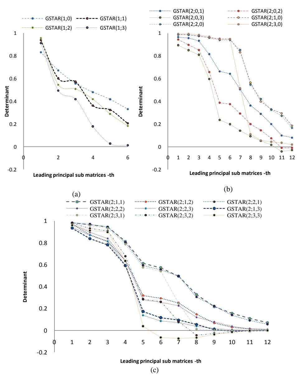
Figure 4 The determinant values of all the leading principal matrices of the IAcM tend to be smaller as the dimensions of the leading principle matrices become larger, (a) possible models with \(1^{st}\) time lag, (b) possible models with \(2^{nd}\) time lag and one of spatial lag is 0, and (c) others possible models with \(2^{nd}\) time lag.
For the forecasting stage, we prepared the ten latest data, collected from January to October 2011. In the advanced checking diagnostic stage, we estimate these data using the five selected models in order to obtain what we call forecast-estimated observations. These forecast-estimated observations will be compared with real observations using (9), so that we have the MSR of the forecast-estimated observations. The results of the MSR can be seen in Table 4.
Table 4 MSR of forecast-estimated of five possible appropriate GSTAR models. The smallest MSR is given by GSTAR(2;3,0) model.
| GSTAR | MSR |
|---|---|
| (1;2) | 175.3843 |
| (1;3) | 139.4374 |
| (2;1,0) | 155.788 |
| (2;2,0) | 141.6173 |
| (2;3,0) | 108.9293 |
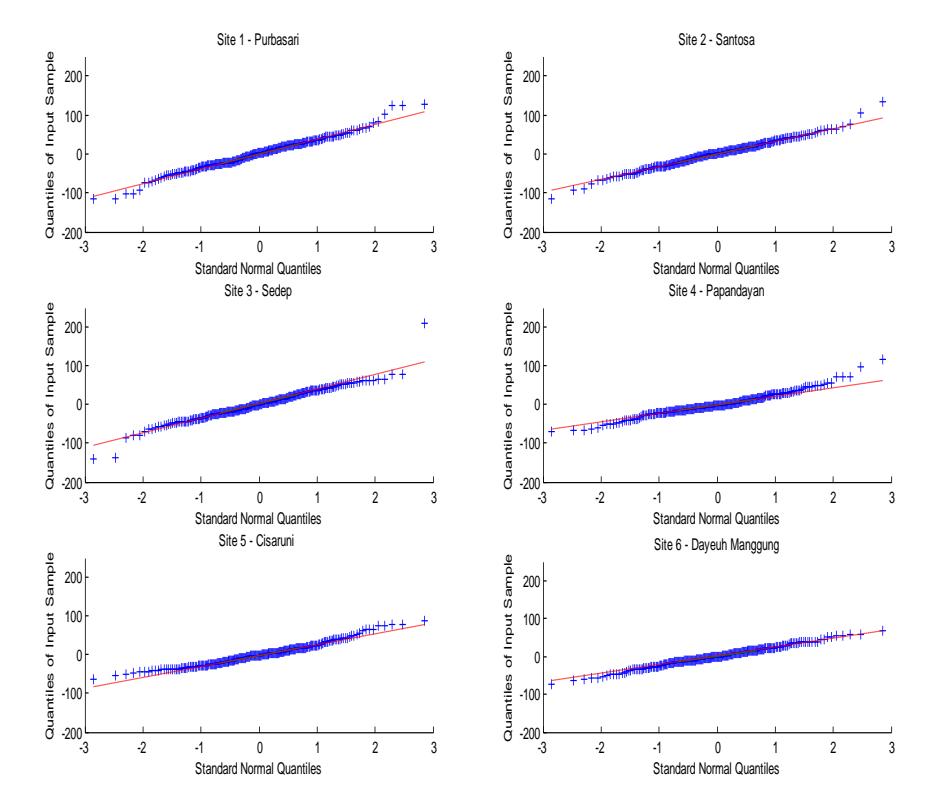
Figure 5 QQ Plot of Sample Data versus Standard Normal Data for each site i, i = 1,2,...,6 (from top left to bottom right). Quantile-quantile plot of the sample quantiles of residuals versus theoretical quantiles from a normal distribution.
Based on the smallest MSR value, we have GSTAR(2;3,0) as the most appropriate model. For convenience, we display a quantile-quantile plot of residuals data versus normal distribution data in Figure 5. Since the plot close to linear, we may say that the residuals have normal distribution.
In order to do forecasting of \((t+1)^{th}\) observations, the GSTAR(2;3,0) may be presented as the following equation.
\[\widehat{\mathbf{Y}}_{t+1} = (\widehat{\mathbf{\Phi}}_{10} + \widehat{\mathbf{\Phi}}_{11} \mathbf{W}^{(1)} + \widehat{\mathbf{\Phi}}_{12} \mathbf{W}^{(2)} + \widehat{\mathbf{\Phi}}_{13} \mathbf{W}^{(3)}) \mathbf{Y}_t + \widehat{\mathbf{\Phi}}_{20} \mathbf{Y}_{t-1}\] (10)
where \(\widehat{\mathbf{Y}}_{t+1}\) is a estimated \((N\times 1)\)-dimensional vector of observations at time t+1, \(\widehat{\mathbf{Y}}_{t+1}=(\widehat{Y}_{1,t+1},\widehat{Y}_{2,t+1},...,\widehat{Y}_{N,t+1})'\), \(\widehat{\boldsymbol{\Phi}}_{1\ell}\) is a estimated \((N\times N)\)-dimensional matrix of autoregressive parameters for the first time lag, with spatial lag \(\ell=0,1,2,3\). The \(\ell=0\) shows the influence of a location on itself.
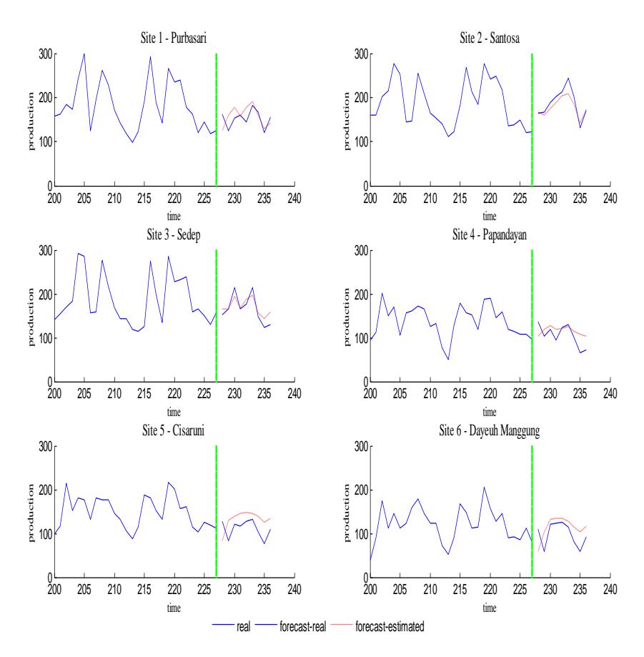
Figure 6 Plot of forecast-estimated observations using GSTAR(2;3,0) model. for each site i, i = 1,2,...,6 (from top left to bottom right).
The GSTAR(2;3,0) model tells us that a location will be influenced by itself until the second time lag, while its neighbors can exert influence during the first time lag within three spatial lags.
The plots of the 28 latest observations and the 10 next forecasted observations, the total MSR of which is 108.9293, are shown in Figure 6. The forecastestimated plots display similar patterns and are close enough to the real observations.
5 Conclusions
An IAcM is suggested to be used in selecting the approriate space-time models in completion of STACF and STPACF values. Using an IAcM decreases the subjectivity of the judgment about which models are appropriate. In the case study of the monthly tea production of six plantations in West Java, we found that GSTAR(2;3,0) is the most appropriate model. We also observed that three types of matrices (uniform, euclidean, and binary) will have the same influence on the modeling process, since the ratio between the number of spatial lags and observed locations is close to one. They are supposed to have different results if the number of observed locationsis much higher than the number of observed spatial lags.
Acknowledgement
The research of the first author was supported by the Fundamental Research of DIKTI DIPA ITB program in 2011. The data were supplied by PT. Perkebunan Nusantara VIII (Persero) in Bandung. The authors are also grateful to Assoc. Prof Wono Setya Budhi and Khreshna Syuhada, Ph.D for their valuable discussions.