
1 Introduction
One important mode of interannual variability in the Indian Ocean is the Indian Ocean Dipole (IOD) [1-3]. A typical positive IOD event is characterized by an east-west dipole pattern in sea surface temperature (SST) anomalies, with negative (positive) SST anomalies observed in the south-eastern (central/ western) tropical region. The SST patterns are associated with a change in the surface winds: easterly (south-easterly) wind anomalies dominate the equatorial (off the coasts of Sumatra and Java) region during the peak phase of the positive IOD event. The changes in the oceanic and atmospheric circulation associated with the positive IOD event cause a westward movement of the convection zone leading to a change in the rain distribution in the surrounding continents [4].
From late summer until fall 2006, a positive IOD event took place in the tropical Indian Ocean. Based on the dipole mode index (DMI), the 2006 IOD event was the strongest of the events in the last 10 years. The evolution of the 2006 IOD event was linked to the equatorial wave dynamics. Using new measurements made in the tropical Indian Ocean, [5] it was shown that the event was preceded by a series of strong upwelling Kelvin waves during latespring and early summer. While an analysis using an ocean general circulation model demonstrated that horizontal advections induced by westward zonal current anomalies contributed to the cooling tendency in the eastern tropical Indian Ocean during June-July 2006 [6].
A recent study highlighted the importance of wind-forced and boundarygenerated equatorial oceanic waves during the evolution of the 2006 IOD event. Three mechanisms have been proposed for the generation of the 2006 IOD event [7]. It was suggested that prior to the event, there was a shoaling of thermocline in the eastern equatorial Indian Ocean, associated with the western boundary-generated upwelling Kelvin waves. This thermocline shoaling was followed by strengthening south-easterly winds during May/June in the southeastern tropical Indian Ocean, leading to net latent heat loss. The anomalous easterly winds in June/July then generated the equatorial upwelling Kelvin waves leading to the development of the 2006 IOD event. Another recent study further highlighted the important role of western-boundary-generated upwelling Kelvin waves associated with upwelling Rossby waves that were generated by westerly wind anomalies during May/June [8].
However, previous studies have only shown qualitatively the important role of equatorial oceanic waves in the evolution of the 2006 IOD event [5-8]. This calls for a quantitative assessment of the role of equatorial waves in the evolution of the 2006 IOD event. In this study, we examine quantitatively the role of equatorial waves in the evolution of the 2006 IOD event, using a winddriven, linear, continuously stratified long-wave ocean model. This model provides the opportunity to identify quantitatively the energy source of these waves during the evolution of the event.
This paper is organized as follows: in Section 2 we describe the data sets and the linear model used; in Section 3 we present the observed evolution of the 2006 IOD and also discuss the role of wind-forced and boundary-generated oceanic waves in the evolution of IOD events using a linear wave model. The final section is reserved for summary and discussion.
2 Data and Method
2.1 Data
Merged satellite sea surface height (SSH) data from Archiving, Validation and Interpretation of Satellite Oceanographic data (AVISO) were used in this study. They cover the period of 14 October 1992 to 22 July 2009, with temporal and horizontal resolutions of 7 days and 0.25°, respectively. The gridded SSH data were obtained from the Ssalto/Duacs multimission altimeter project (http://www.aviso.oceanobs.com). Surface winds were obtained from the QSCAT daily winds, which are available on a 0.25°×0.25° grid, from 19 July 1999 to 29 October 2009. Sea surface temperature (SST) data were derived from Tropical Rain Measuring Mission (TRMM) data with a weekly resolution on a 0.25°×0.25° grid, from January 1998 to December 2009. QSCAT wind and SST data were provided by Remote Sensing Systems (http://www.remss.com).
In addition, near-surface velocity data from the Ocean Surface Current Analysis Real-time (OSCAR) project were used [9], representing oceanic flow at a depth of 15 m. This product is derived from satellite SSH, surface winds and drifter data using a diagnostic model of ocean currents based on frictional and geostrophic dynamics. The data are available from 21 October 1992 to 1 September 2010, with a horizontal resolution of 1°×1° and a temporal resolution of 5 days.
Mean climatologies for SSH, SST, winds and surface current were calculated from time series over the period of January 2000 to December 2008, for which all data are available. Then, anomaly fields for all variables were constructed on the basis of deviations from their mean climatology. Finally, the anomalous data were smoothed with a 15-day running mean filter.
2.2 Method
In order to evaluate the role of equatorial oceanic waves in the evolution of the 2006 IOD event, we used a linear-stratified ocean model. The model is based on a method of characteristics for solving wind-forced Kelvin waves and long Rossby waves [10,11]. Following [12], the momentum and continuity equation for the vertical baroclinic mode are written with a long-wave approximation as
\[u_{nt} + \frac{A}{c_n^2} u_n - \beta y v_n + p_{nx} = \frac{\tau^x}{\rho \int_{-D}^0 \psi_n^2 dz}\] (1)
\[\beta y u_n + p_{ny} = \frac{\tau^y}{\rho \int_{-D}^0 \psi_n^2 dz}\] (2)
\[p_{nt} + Ap_n + c_n^2 \left( u_{nx} + v_{ny} \right) = 0, \tag{3}\] where subscripts t, x, y indicate the derivative function, (u, v) are the zonal and meridional velocities, p is pressure, \(c_n\) is the eigenvalue of the nth vertical mode, A is a constant referring to friction or diffusion, \(\beta\) is the gradient of the Coriolis parameter, \(\psi_n\) is the nth vertical structure function, \((\tau^x, \tau^y)\) are the zonal and meridional surface winds, and D is the ocean depth.
The solution for wind-forced oceanic equatorial Kelvin waves (with m = 1) can be expressed as
\[u_{nm} = \zeta_{nm}(x, z, t)\phi_0(y) \tag{4}\]
\[p_{mn} = c_n \zeta_{mn}(x, z, t) \phi_0(y). \tag{5}\]
Similarly, the solution for wind-forced oceanic Rossby waves (with \(m \ge 1\)) is written as
\[u_{mn} = \varsigma_{mn}(x, z, t) \left( \sqrt{\frac{m}{m+1}} \phi_{m+1}(y) - \phi_{m-1}(y) \right)\] (6)
\[p_{mn} = c_n \varsigma_{mn}(x, z, t) \left( \sqrt{\frac{m}{m+1}} \phi_{m+1}(y) - \phi_{m-1}(y) \right), \tag{7}\] where m is the meridional mode number and \(\phi_m\) is a Hermite function of order m. \(\zeta_{mn}\) (x,z,t) is any dependent variable (velocity or pressure) represented by the integration of the wind projection onto one of the modes,
\[\varsigma_{mn}(x,z,t) = \varsigma_{mn} \left[ X, t + \frac{(X-x)}{c_n} \right] + \alpha_n(z) \int_X^x B_{mn} \left[ \xi, t \right] + \frac{(\xi - x)}{c_n} \times \exp\left[ -r_n(x - \xi) \right] d\xi.\] (8)
Here, X is the eastern (western) boundary for the Rossby (Kelvin) waves, and \(r_n\) represents a damping coefficient. \(\alpha_n(z)\) is an amplitude of coefficient which is represented by
\[\alpha_n^u(z) = \frac{\psi_n(0)\psi_n(z)}{\rho c.D},\tag{9}\]
\[\alpha_n^P(z) = \frac{\psi_n(0)\psi_n(z)}{\rho D}.\] (10)
The term Bmn in (7) is the projection coefficient of the wind onto one of the wave modes. For the Kelvin wave, it is represented as
\[B_{-1n} = \frac{1}{\sqrt{2}} \int \frac{\phi_0(y)\tau^x(x, y, t)}{(c_n / \beta)^{1/2}},\] (11)
while for the Rossby wave, it is written as
\[B_{mn} = \int_{-\infty}^{+\infty} \left[ \frac{\phi_{m+1}(y)}{\sqrt{m+1}} - \frac{\phi_{m-1}(y)}{\sqrt{m}} \right] \frac{\tau^{x}(x, y, t)}{(c_{n} / \beta)^{1/2}} dy.\] (12)
Thus, the total ocean response to the wind forcing is the sum of all these waves, which is written as
\[R = \sum_{n=1}^{\infty} \left( \sum_{m=1}^{\infty} \varsigma_{mn} + \varsigma_{-1n} \right). \tag{13}\]
The model retains the first 10 baroclinic modes and 15 meridional modes (the Kelvin mode and the first 14 Rossby modes). Vertical modes are calculated using a mean density stratification from the observed Argo temperature and salinity from surface to 4000 m, averaged over the region of 15°S–15°N and 40°E–100°E. Phase speeds for the first and second baroclinic mode Kelvin waves are 2.5 and 1.55 m s<sup>-1</sup>, respectively, in agreement with previous studies in the equatorial Indian Ocean [12,13].
The model is unbounded in the meridional direction, and the zonal domain spans 40°E–100°E, with straight north-south meridional walls at the eastern and western boundaries. The reflection efficiency at both the eastern and western boundary is set to 85% following observational results [14]. The grid sizes are \(\Delta x = 2^{\circ}\) and \(\Delta t = 12\) hours. The damping coefficient is \(A/c_n^2\), where c is the phase speed of the baroclinic Kelvin wave and subscript n denotes the vertical mode number. The parameter A is an arbitrary constant, which is chosen so that the damping coefficient for the first vertical baroclinic mode is (12 months)-1 . The model is forced for the period of 1 January 1980 to 30 April 2010, with daily wind stresses from the European Centre for Medium Range Forecasting (ECMWF). Despite the idealization of the eastern and western boundaries applied in the model, it reproduces successfully the observed variability of seasonal and interannual sea levels and zonal currents in the equatorial Indian Ocean [10,11].
3 Results
3.1 Observed Evolution of the 2006 Indian Ocean Dipole
Figure 1 shows the evolution of the Dipole Mode Index (DMI) and Niño3.4 Index from January 2006 through February 2007. The SST anomaly in the eastern and western Indian Ocean shows a normal condition during January-July 2006 (Figure 1a). Similarly, the Pacific Ocean was also in a normal condition (Figure 1b).
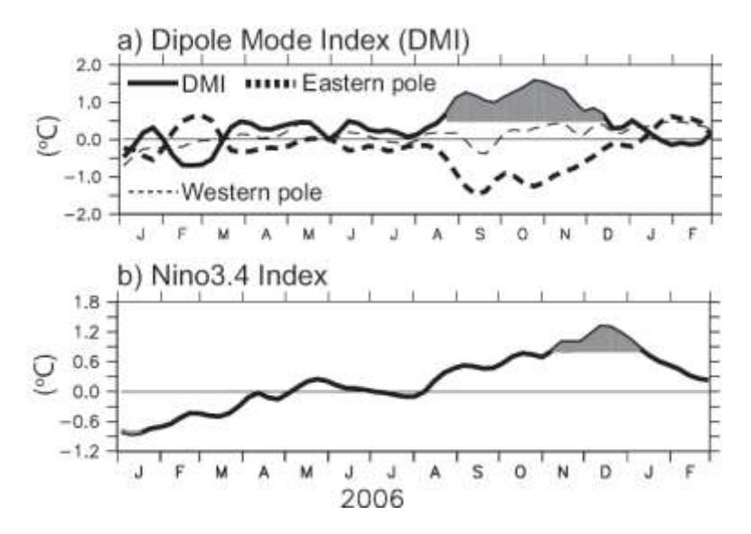
Figure 1 Time series of (a) Dipole Mode Index (DMI) and (b) Niño3.4 Index from January 2006 to February 2007. The DMI is defined as the difference in SST anomaly between the western region (50E70E, 10S10N) and the eastern region (90E110E, 10SEquator). The Niño3.4 Index is defined as an averaged SST anomaly in the region bounded by 5°N–5°S, 170°W–120°W. Values larger than one standard deviation are highlighted in gray.
The evolution of the IOD started in August 2006 when the DMI rapidly increased, associated with a cooling in the eastern Indian Ocean (Figure 1a). After a warming tendency in late September 2006, the DMI again increased and reached its maximum of about 1.5 C in late October 2006. The increase of the DMI co-occurred with a warming tendency in the western pole that started in late September and continued until November.
The DMI rapidly diminished in late October, which was associated with a rapid warming of the eastern pole (Figure 1a). The IOD completely disappeared in early December, when the SST anomaly returned to a normal condition. At the same time, in the Pacific Ocean the evolution of the El Niño event reached its peak (Figure 1b). However, the Niño3.4 Index rapidly decreased thereafter. A discussion of the evolution of the 2006 El Niño event is beyond the topic of this study; we only note that the 2006 IOD event co-occurred with a weak El Niño event.
3.2 The Role of Equatorial Waves
The evolution of the IOD event was controlled by the equatorial ocean dynamics [1,15-17]. Upwelling equatorial Kelvin waves generated by easterly anomalies lift the thermocline in the eastern Indian Ocean, and anomalous south-easterly winds along the coast of Sumatra enhance the cooling in the eastern Indian Ocean [3]. In the western Indian Ocean, early studies have demonstrated that downwelling off-equatorial Rossby waves associated with an easterly wind anomaly could deepen thermocline and induce warm SST in the western Indian Ocean [15-17].
In order to examine the role of the equatorial oceanic waves in the evolution of the 2006 IOD event, the time-longitude sections of zonal wind stress, zonal surface currents and SSH anomalies along the equator, and the SSH anomaly along 5S are presented in Figures 2a, 2b, 2c, and 2d, respectively. During January-May 2006, there was an alternate change between westerly and easterly winds along the equator (Figure 2a) which generated eastward and westward near-surface zonal currents along the equator (Figure 2b). In addition, these westerly and easterly winds also forced downwelling (positive SSH anomaly) and upwelling (negative SSH anomaly) along the equator (Figure 2c). At the same time, we also observed upwelling and downwelling in the off-equatorial region, centered along ~5S, consistent with the signs of equatorial wind anomalies and equatorial wave theory (Figure 2d).
Interestingly, prior to the occurrence of the IOD, we observed a series of eastward propagating positive (K1) and negative (K2) SSH signals along the equator (Figure 2c). The positive signals observed in June closely corresponded to the westerly wind anomalies along the equator (Figure 2a) that also forced eastward zonal currents (Figure 2b). From late July through August, the winds reversed to easterly anomalies (Figure 2a). As a result, the zonal currents became westward (Figure 2b) and there were eastward propagating negative SSH anomalies along the equator during this time (Figure 2c). Early studies reported that these westward zonal current anomalies played a significant role in the cooling tendency of the eastern equatorial Indian Ocean at the onset of the 2006 IOD event [6,7,18]. This suggests an important role of the equatorial oceanic waves in the activation of the 2006 IOD, which we turn to in the following sub-section.
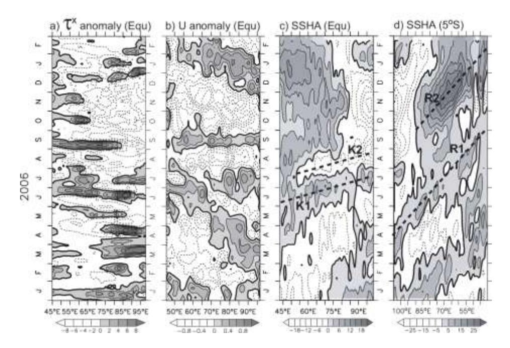
Figure 2 Time-longitude diagrams of (a) zonal wind stress anomalies, (b) zonal current anomalies, and (c) sea surface height anomalies along the equator, and (d) sea surface height anomalies along 5S. Contour intervals are 2 10-2 N/m2 , 0.2 m/s, 3 cm, 5 cm in (a), (b), (c) and (d), respectively. Positive anomalies are shaded and the zero contour is highlighted with a thick line. Note that scales change in each panel, and the x-axis in (d) is flipped to evidence the reflection in the eastern boundary.
After a short reversal of the zonal wind anomalies in September, the winds were dominated by easterly wind anomalies from October through December (Figure 2a). In response to these easterly wind anomalies, the zonal currents became westward (Figure 2b). Moreover, the SSH anomalies indicated a typical dipole
pattern with negative anomalies observed in the eastern region and positive anomalies loading in the western region (Figure 2c).
In the off-equatorial region, we observed robust westward propagating positive SSH anomalies (R1) that moved across the basin from April to August/September (Figure 2d). Part of these signals seemed to originate from the eastern boundary reflection generated by incoming downwelling signals in the eastern boundary during March-April (Figure 2c). This may suggest the importance of the boundary-generated oceanic waves in generating positive SSH anomalies in the western boundary.
During the peak phase of the IOD, we observe strong positive SSH anomalies (R2) that propagated westward (Figure 2d). These signals corresponded to the easterly wind anomalies along the equator during October-December (Figure 2a) that caused upwelling (negative SSH anomalies) along the equator east of about 75E, and downwelling (positive SSH anomalies) in the off-equatorial region west of about 85E (Figures 2c,d).
3.3 Model Wind-Forced and Boundary-Generated Oceanic Waves
In order to evaluate the role of wind-forced and boundary generated waves in forcing zonal currents and SSH anomalies during the activation phase of the 2006 IOD event, we turn to the results of the linear wave model. First, we compare the results of the model with the observations in Figure 3. The model well reproduces the zonal currents and SSH anomalies associated with the evolution of the 2006 IOD event. The westward zonal currents and negative SSH anomalies in August during the onset of the 2006 IOD event are well captured by our model (Figures 3a-b, 3d-e). In the off-equatorial region, our model also reproduces the westward propagating positive SSH anomalies during April-August and during the peak phase of the IOD event in October-December (Figures 3c, 3f). However, the model's zonal currents and SSH anomalies are weaker compared to the observations. The weaker amplitude in the model is partially caused by the model's simplified coastline. In addition, the lack of coastal wave dynamics may also contribute to this discrepancy.
One of the main advantages of using a linear wave model is that the relative importance of wind-forced and boundary-generated waves can be diagnosed separately. Figure 4 shows the contributions of wind-forced and boundary generated waves to the zonal current anomalies along the equator during January 2006 through February 2007.
Apparently, the westward zonal current anomalies observed during the onset of the IOD in August mainly resulted from the wind-forced Kelvin waves (Figure 4b). Short-term eastward zonal current anomalies appeared along the equator in September (Figure 4e) and were also influenced by the wind-forced Kelvin waves (Figure 4b), though the reflected Rossby waves (Figure 4c) played a dominant role in generating eastward zonal current anomalies near the eastern boundary.
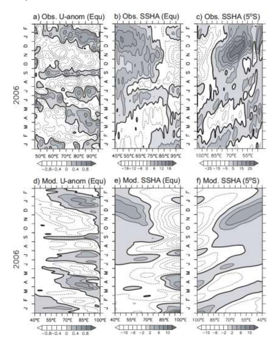
Figure 3 (a-c) same as for Figures 2b-d. (d-f) same as in (a-c), except output from the simulation model. Note that scales change in each panel, and the x-axis in (c) and (f) is flipped to evidence the reflection at the eastern boundary.
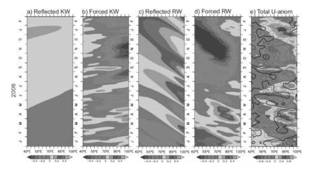
Figure 4 Time-longitude diagrams of model zonal current anomalies along the equator for January 2006-February 2007. (a) reflected Kelvin waves, (b) windforced Kelvin waves, (c) reflected Rossby waves, (d) wind-forced Rossby waves, and (e) total. The contours in (e) show anomalies of zonal wind stress along the equator. The solid (dotted) lines are for westerly (easterly) anomalies. The contour interval is 2 10-2 N/m2 with the zero contour highlighted. Note the scale changes in (e).
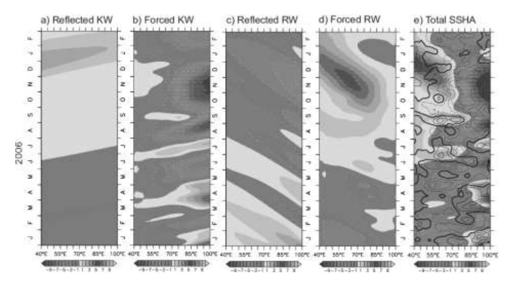
Figure 5 Same as Figure 4, except for the sea surface height anomalies along the equator.
The role of the equatorial oceanic waves in generating SSH anomalies is presented in Figure 5. It shows clearly that the wind-forced Kelvin waves (Figure 5b) significantly contributed to generating negative SSH anomalies at the onset of the IOD in August (Figure 5e). A short reversal of the zonal wind anomalies during September (Figure 5e) excited downwelling Kelvin waves (Figure 5b). However, the signals resulting from the wind-forced Kelvin waves were much weaker than the total solution (Figure 5e). We found that windforced Rossby waves made a significant contribution to the elevated sea levels in the western basin during this time (Figure 5d).
The results of the model suggest that the upwelling equatorial waves (negative SSH anomalies) and westward zonal current anomalies that contributed to significant sea surface cooling in the eastern equatorial Indian Ocean during the activation phase of the 2006 IOD event were mainly generated by wind-forced Kelvin waves.
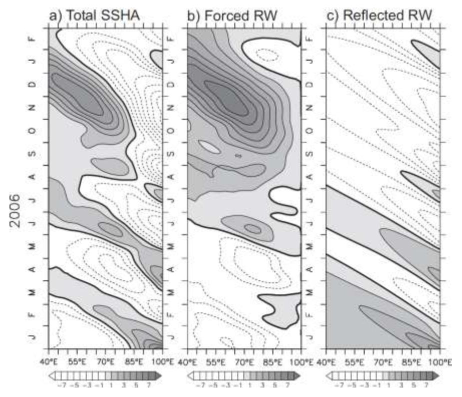
Figure 6 Simulated sea level variations along 5S during January 2006- February 2007 from (a) total solution, (b) wind-forced Rossby waves, and (c) reflected Rossby waves. Positive anomalies are shaded and the zero contour is highlighted with a thick line. The contour interval is 1 cm.
As demonstrated in the previous studies, off-equatorial Rossby waves play an important role in generating SSH and zonal current variability in the western Indian Ocean [15-17]. Here, we focus only on the SSH variations in the offequatorial region. Figure 6 shows the contribution of wind-forced and boundary generated Rossby waves on the SSH variations along 5S. Our model indicates that elevated sea levels in the western boundary during the activation of the 2006 IOD event in July-August (Figure 6a) were due to both wind-forced and boundary-generated Rossby waves (Figures 6b,c). The wind-forced downwelling Rossby waves were associated with the easterly wind anomalies along the equator in June (Figure 2a) that caused anomalous surface divergence along the equator east of about 55E (Figures 2c, 3e), and anomalous surface convergence in the off-equatorial region west of about 85E (Figures 2d, 3f). On the other hand, the boundary-generated downwelling Rossby waves originated from the reflection of downwelling equatorial Kelvin waves that reflected from the eastern boundary in March- April 2006 (2c). Thus, the model suggests that a complex interplay of wind-forced and boundary-generated downwelling Rossby waves elevated sea levels in the western equatorial Indian Ocean during the activation phase of the 2006 IOD event.
4 Discussion
The elevated sea levels in the western equatorial Indian Ocean during the activation phase of the 2006 IOD event resulted from a complex interplay of wind-forced and boundary-generated downwelling Rossby waves. The windforced downwelling Rossby waves were associated with the easterly wind anomalies along the equator observed in June (Figure 6b). These anomalous winds caused anomalous surface divergence along the equator east of about 55E and anomalous surface convergence in the off-equatorial regions west of about 85E. On the other hand, the boundary-generated downwelling Rossby waves were generated by the eastern-boundary reflection of downwelling equatorial Kelvin waves that arrived in the eastern boundary in March-April 2006 (Figure 6c).
These results agree with a previous study, which shows the importance of equatorial Kelvin waves for the development of the cooling tendency in the eastern equatorial Indian Ocean during the activation of the 2006 IOD event [5]. Our results also show that the western-boundary-generated waves only played a minor role during the activation of the event, in contrast to previous studies [7,8]. One should note that the analysis in these studies was based only on the SSH variations [7,8].
[7] has shown that the cooling tendency in the eastern equatorial Indian Ocean in June 2006 was mainly due to surface heat flux, since the zonal heat advections were nearly zero at that time. Our model reveals that the boundarygenerated Rossby waves originated from upwelling equatorial Kelvin waves and forced eastward zonal currents during June [Figure 5c,e]. This may have resulted in a weak contribution of the zonal heat advection on the cooling tendency in the eastern equatorial Indian Ocean in June. In addition, the presence of strong anomalous westerly wind anomalies along the equator from late June to early July excited strong downwelling Kelvin waves that warmed the eastern equatorial Indian Ocean and canceled the previous cooling tendency, in agreement with previous studies [18].
5 Conclusion
The role of equatorial oceanic waves in activating the 2006 IOD event was evaluated on the basis of observations and outputs from a linear wave model. The model is continuously stratified, and the longwave approximation has been used so that only the Kelvin and the Rossby modes are retained. The model is unbounded in the meridional direction, and it has meridional walls along 40E and 100E. The model is forced by the ECMWF winds from 1980 through 2010.
Our analysis found that anomalous easterly winds along the equator during the activation phase of the 2006 IOD event in August generated upwelling Kelvin waves and westward near-surface zonal currents which contributed to significant sea surface cooling in the eastern equatorial Indian Ocean (Figures 4b, 5b).
Acknowledgments
The author would like to thank Dr. Motoki Nagura for the model output. This study is supported by the Indonesia Toray Science Foundation (ITSF) Research Grant 2012 and by the University of Sriwijaya through Penelitian Unggulan Universitas 2012. This is CGCCS contribution number 1201.