
1 Introduction
A very informative way of specifying the accuracy of a time series prediction is to use a prediction interval. To do this, some authors, e.g. [1-5], have computed the prediction interval or limit for the autoregressive (AR) process and the autoregressive conditional heteroscedastic (ARCH) process. For these models, they have assumed that the fitted model is the true model. In other words, the authors have employed properly specified models.
In practice, however, time series models are likely to be misspecified. For instance, an AR(1) model is fitted but the true model is an AR(2) or MA(1) model. This paper deals with the prediction interval in the case of a misspecified AR(1) model. In the context of the prediction problem, there have been a few papers, such as [6] and [7], that provide derivations of expressions for meansquared-error of prediction in the case of a misspecified Gaussian AR(p) model. An investigation of the coverage probability, conditional on the last observations, of a prediction interval based on a misspecified Gaussian AR(p) model was presented first by [8].
In the case of a misspecified Gaussian AR(p) model, the derivation of the asymptotic expansion of the coverage probability, conditional on the last
observations, of a prediction interval requires a great deal of care. To make clear the issues involved in this derivation, we consider the simple scenario described in Section 2. Namely, a misspecfied zero-mean Gaussian AR(1) process fitted to a stationary zero-mean Gaussian process. We also consider a one-step-ahead prediction interval with target coverage probability. Similarly to [8], we aim to find the asymptotic expansion for the coverage probability of the prediction interval under consideration, conditional on the last observation.
In Section 3, we compute the conditional coverage probabilities for both properly and misspecified first order autoregressive models. This is aimed to examine the effect of misspecification on the coverage probability of the prediction interval. Furthermore, the technical argument for finding the conditional coverage probability of a prediction interval as proposed by de Luna (which differs from the estimative prediction interval) is reviewed in detail in Section 4. A numerical example to illustrate a gap in his argument is given in Section 5.
2 Description of the Time Series and Fitted Models
Consider a discrete time stationary Gaussian zero-mean process \(\{Y_t\}\). Let \(\gamma_k = E(Y_t Y_{t-k})\) denote the autocovariance function of \(\{Y_t\}\) evaluated at lag k. Suppose that \(\sum_{j=1}^{\infty} |\gamma_j| < \infty\). We do not require that \(\{Y_t\}\) is an AR(1) process. The available data are \(Y_1, Y_2, \ldots, Y_n\). We will be careful to distinguish between random variables, written in upper case, and their observed values, written in lower case.
We consider one-step-ahead prediction using a stationary Gaussian zero-mean AR(1) model. This model may be misspecified. Let \(\rho_k = \gamma_k/\gamma_0\). Define \(\theta\) to be the value of a that minimizes \(E(Y_{n+1}-aY_n)^2\). Thus \(\theta=\gamma_1/\gamma_0\). Define \(\psi^2=var(Y_{n+1}|Y_n=y_n)\). Note that
\[\psi^2 = \gamma_0 - \frac{\gamma_1^2}{\gamma_0}\] and \(E(Y_{n+1}-\Theta Y_n)^2=\psi^2\). Let \(\widehat{\Gamma}_k\) denote a consistent estimator of \(\gamma_k\) such as \(n^{-1}\sum_{j=k+1}^n Y_j Y_{j-k}\). Let \(\widehat{\Theta}=\widehat{\Gamma}_1/\widehat{\Gamma}_0\) and note that \(\widehat{\Theta}\) is a consistent
estimator of \(\theta\). We use the notation \([a\pm b]\) for the interval [a-b,a+b] (b>0).
3 The Coverage Properties of Misspecified AR(1) Model
In this section, we examine the effect of misspecification on the coverage probability of the prediction interval. The true model \(\{Y_t\}\) is a zero-mean Gaussian AR(2) process, satisfying
\[Y_{t} = \theta_{1} Y_{t-1} + \theta_{2} Y_{t-2} + \eta_{t} \tag{1}\] for all integer t, where \(\eta_t\) are independent and identically \(N(0, \sigma^2)\) distributed. The roots of \(1 - \theta_1 m - \theta_2 m^2\) are outside the unit circle to ensure stationarity of the process.
We consider an upper one-step-ahead prediction interval with conditional mean square prediction error equal to \(V^2\), i.e.
\[I_{u}(Y_{n};\Theta,V) = \Theta Y_{n} + \Phi^{-1}(1-\alpha)V,\] (2)
where the estimators \(\widehat{\Theta}\) and \(\widehat{V}\) are obtained by maximizing the loglikelihood function conditional on \(Y_1 = y_1\), that are
\[\widehat{\Theta} = \frac{\sum_{t=1}^{n-1} Y_t Y_{t+1}}{\sum_{t=1}^{n-1} Y_{t+1}^2}\] and
\[\widehat{V}^{2} = \frac{1}{n-1} \sum_{t=1}^{n-1} (Y_{t} - \widehat{\theta} Y_{t+1})^{2}.\]
The coverage probability of \(I_u(Y_n; \Theta, V)\), conditional on \(Y_n = y_n\) is calculated as follows. First, we observe that
\[P(Y_{n+1} \leq \widehat{\Theta} Y_n + \Phi^{-1}(1-\alpha)\widehat{V} | Y_n = y_n, Y_{n-1} = y_{n-1})\] \[= P(\theta_1 Y_n + \theta_2 Y_{n-1} + \eta_{n+1} \leq \widehat{\Theta} Y_n + \Phi^{-1}(1-\alpha)\widehat{V} | Y_n = y_n, Y_{n-1} = y_{n-1})\] \[= P(\eta_{n+1} \leq (\widehat{\Theta} - \theta_1) y_n - \theta_2 y_{n-1} + \Phi^{-1}(1-\alpha)\widehat{V} | Y_n = y_n, Y_{n-1} = y_{n-1})\] \[= E\left(\widehat{\Theta} - \widehat{\theta}_1 \frac{y_n}{\sigma} - \theta_2 \frac{y_{n-1}}{\sigma} + \Phi^{-1}(1-\alpha) \frac{\widehat{V}}{\sigma} | Y_n = y_n, Y_{n-1} = y_{n-1}\right)\] (3)
and we estimate this conditional expectation by simulation. We use the backward representation:
\[Y_{t} = \theta_{1} Y_{t+1} + \theta_{2} Y_{t+2} + V_{t} \tag{4}\] for all integer t, where \(V_t\) are independent and identically \(N(0, \sigma^2)\) distributed. It is noted that \(V_t\) and \(Y_{t+1}, Y_{t+2}, \ldots\) are independent. We begin the simulation run by setting \((Y_n, Y_{n-1}) = (y_n, y_{n-1})\) and then use (4) to run the process backwards in time.
Table 1 Estimated coverage probabilities, conditional on \((Y_n, Y_{n-1}) = (0,1)\), of the upper 0.95 one-step-ahead forecasting intervals for true and misspecified models. Standard errors are in brackets.
| \(a_1, a_2, \sigma^2\) | Model | ||
|---|---|---|---|
| \(a_1 = 1, a_2 = 0.25, \sigma^2 = 1\) | True | 0.9401 | 0.9451 |
| 1 2 7 | (0.00079) | (0.00055) | |
| Misspecified | 0.9999 | 1 (0.000002) | |
| _ | (0.00001) | ||
| \(a_1 = 0.1, a_2 = -0.4, \sigma^2 = 1\) | True | 0.9327 | 0.9423 |
| 1 / 2 / | (0.00091) | (0.00056) | |
| Misspecified | 0.9311 | 0.9316 | |
| - | (0.0011) | (0.0009) | |
| \(a_1 = -0.3, a_2 = -0.3, \sigma^2 = 1\) | True | 0.9342 | 0.9419 |
| ,,,,,,,,,,,,,,,,,,,,,,,,,,,,,,,,,,,,,,,,,,,,,,,,,,,,,,,,,,,,,,,,,,,,,,,,,,,,,,,,,,,,,,,,,,,,,,,,,,,,,,,,,,,,,,,,,,,,,,,,,,,,,,,,,,,,,,,,,,,,,,,,,,,,,,,,,,,,,,,,,,,,,,,,,,,,,,,,,,,,,,,,,,,,,,,,,,,,,,,,,,,,,,,,,,,,,,,,,,,,,,,,,,,,,,,,,,,,,,,,,,,,,,,,,,,,,,,,,,,,,,,,,,,,,,,,,,,,,,,,,,,,,,,,,,,,,,,,,,,,,,,,,,,,,,,,,,,,,,,,,,,,,,,,,,,,,,,,,,,,,,,,,,,,,,,,,,,,,,,,,,,,,,,,,,,,,,,,,,,,,,,,,,,,,,,,,,,,,,,,,,,,,,,,, | (0.00088) | (0.00057) | |
| Misspecified | 0.9656 | 0.9728 | |
| • | (0.0010) | (0.0007) | |
| \(a_1 = -0.75, a_2 = 0.5, \sigma^2 = 1\) | True | 0.9427 | 0.9468 |
| (0.00074) | (0.00049) | ||
| Misspecified | 0.9988 | 0.9993 | |
| • | (0.00006) | (0.00002) |
Table 1 presents the estimate of conditional coverage probability (3). Standard errors of these estimates are given in brackets. We also provide the estimate of conditional coverage probability of when the predictor is also a zero-mean Gaussian AR(2) model (properly specified model) as in [4].
4 The Conditional Distribution for Misspecified Model
de Luna [8] considers the data generating mechanism \(\{Y_t\}\), as described earlier, and h-step-ahead prediction using a zero-mean Gaussian AR(p) model. This model may be misspecified. Consider the case that h=1 and p=1. His \(1-\alpha\) prediction interval for \(Y_{n+1}\) is
\[J = [\widehat{\Theta}Y_n - \sqrt{\psi^2 + \omega^2(Y_n)} z_{1-\alpha/2}, \widehat{\Theta}Y_n + \sqrt{\psi^2 + \omega^2(Y_n)} z_{1-\alpha/2}],\] where \(\omega^2(Y_n) = n^{-1}wY_n^2\), \(w = \sum_{k=1}^{\infty} (\rho_{k+1} + \rho_{k-1} - 2\rho_1\rho_k)^2\) and \(z_{1-\alpha/2}\) is the \((1-\alpha/2)\) quantile of the N(0,1) distribution. In practice, \(\psi^2\) and w are unknown since they depend on an unknown autocovariance function of the process \(\{Y_k\}\). However, de Luna assumes that both \(\psi^2\) and w are known.
de Luna claims that \(P(Y_{n+1} \in J | Y_n = y_n) = 1 - \alpha + O(n^{-1})\). His justification for this claim, with intermediate steps added, is the following.
\[P(Y_{n+1} \in J | Y_n = y_n)\] \[= P(Y_{n+1} \in [\Theta y_n \pm \sqrt{\psi^2 + \omega^2(y_n)} z_{1-\alpha/2}] | Y_n = y_n)\] (by the substitution theorem for conditional expectations) \[= E(P(Y_{n+1} \in [\Theta y_n \pm \sqrt{\psi^2 + \omega^2(y_n)} z_{1-\alpha/2}] | Y_n = y_n, \Theta) | Y_n = y_n),\] by the double expectation theorem. To evaluate this conditional expectation, de Luna proceeds as follows. Define \(F(\cdot)\) and \(f(\cdot)\) to be the cdf and pdf of \(Y_{n+1}\) conditional on \(Y_n = y_n\), respectively. He then assumes that
\[P(Y_{n+1} \in [\Theta y_n \pm \sqrt{\psi^2 + \omega^2(y_n)} z_{1-\alpha/2}] | Y_n = y_n, \Theta)\] is equal to
\[\widehat{F(\Theta y_n} + \sqrt{\psi^2 + \omega^2(y_n)} z_{1-\alpha/2}) - \widehat{F(\Theta y_n} - \sqrt{\psi^2 + \omega^2(y_n)} z_{1-\alpha/2}), \quad (5)\]
since the Taylor expansions are applied to F and not some other function. Then, by Taylor expansion of F around \(\theta y_n + \psi z_{1-\alpha/2}\),
\[\widehat{F(\Theta y_n + \sqrt{\psi^2 + \omega^2(y_n)} z_{1-\alpha/2})}\] \[= F(\theta y_n + \psi z_{1-\alpha/2})\] \[+ f(\theta y_n + \psi z_{1-\alpha/2})(y_n(\Theta - \theta) + (\sqrt{\psi^2 + \omega^2(y_n)} - \psi)z_{1-\alpha/2}) + \cdots\]
Now, \(F(\theta y_n + \psi z_{1-\alpha/2}) = 1 - \alpha/2\). Thus
\[E(F(\widehat{\Theta}y_n + \sqrt{\psi^2 + \omega^2(y_n)}z_{1-\alpha/2})|Y_n = y_n)\] is equal to
\[1 - \frac{\alpha}{2} + f(\theta y_n + \psi z_{1-\alpha/2})(y_n E(\Theta - \theta | Y_n = y_n) + (\sqrt{\psi^2 + \omega^2(y_n)} - \psi)z_{1-\alpha/2}) + \cdots\]
Similarly,
\[\begin{split} E(F(\widehat{\Theta}y_n - \sqrt{\psi^2 + \omega^2(y_n)} \, z_{1-\alpha/2}) | Y_n &= y_n) \\ &= \frac{\alpha}{2} + f(\theta y_n - \psi z_{1-\alpha/2}) (y_n E(\widehat{\Theta} - \theta \, | \, Y_n = y_n) - (\sqrt{\psi^2 + \omega^2(y_n)} - \psi) z_{1-\alpha/2}) + \cdots \\ \text{If it is assumed that } \widehat{E(\widehat{\Theta} - \theta \, | \, Y_n = y_n)} &= O(n^{-1}) \quad \text{then} \\ P(X_{n+1} \in J | Y_n = y_n) &= 1 - \alpha + O(n^{-1}) \, . \end{split}\]
The assumption (5) is crucial. It is true if \(\{Y_t\}\) is also an AR(1) process (i.e. if the model is properly specified), but it is not necessarily true if the model is misspecified. Let \(F^{\dagger}(\cdot;\hat{\theta})\) denote the cdf of \(Y_{n+1}\) conditional on \(Y_n = y_n\) and
\[\hat{\Theta} = \hat{\theta}\]. Now
\[\begin{split} P(Y_{n+1} \in [\overset{\frown}{\Theta} y_n \pm \sqrt{\psi^2 + \omega^2(y_n)} \, z_{1-\alpha/2}] | \, Y_n &= y_n, \overset{\frown}{\Theta}) \\ &= F^\dagger(\overset{\frown}{\Theta} y_n + \sqrt{\psi^2 + \omega^2(y_n)} \, z_{1-\alpha/2}; \overset{\frown}{\Theta}) - F^\dagger(\overset{\frown}{\Theta} y_n - \sqrt{\psi^2 + \omega^2(y_n)} \, z_{1-\alpha/2}; \overset{\frown}{\Theta}). \end{split}\] If \(\{Y_t\}\) is also an AR(1) process then, by the Markov property, \(F^\dagger(\cdot; \hat{\theta}) = F(\cdot)\) and so (5) is satisfied. If, however, the model is misspecified then \(F^\dagger(\cdot; \hat{\theta})\) is not necessarily equal to \(F(\cdot)\).
5 Computational Example to Illustrate the Error in the Calculating Conditional Distribution
In this section, we provide a numerical example to support the following argument. For a misspecified AR(1) model, the distribution of \(Y_{n+1}\) conditional on \(Y_n = y_n\) is not identical to the distribution of \(Y_{n+1}\) conditional on \(Y_n = y_n\) and \(\Theta = \hat{\theta}\). In doing so, we seek an estimator \(\Theta\), an observed value \(\hat{\theta}\) and a misspecified AR(1) model such that the condition \(\Theta = \hat{\theta}\), when added to the condition \(Y_n = y_n\), tells us a great deal more about the value of \(Y_{n+1}\) than the condition \(Y_n = y_n\) alone.
Consider the following estimator:
\[\widehat{\Theta} = \frac{\left(\sum_{t=2}^{T} Y_{t} Y_{t-1}\right)^{2}}{\sum_{t=2}^{T} Y_{t}^{2} \sum_{t=2}^{T} Y_{t-1}^{2}}\] (6)
and let \((y_1,...,y_n) = (Y_2,...,Y_T)\) and \((x_1,...,x_n) = (Y_1,...,Y_{T-1})\). Thus, we write the estimator (6) as
\[\widehat{\Theta} = \frac{\left(\sum_{i=1}^{n} y_i x_i\right)^2}{\sum_{i=1}^{n} y_i^2 \sum_{j=1}^{n} x_j^2}\] which is less than or equal to 1, according to the Cauchy-Schwarz inequality. Equality occurs if \(x_i = a^* y_i\), i.e. \(Y_t = a^* Y_{t+1}\), where
\[a^* = \frac{\sum_{i=1}^n y_i x_i}{\sum_{i=1}^n y_i^2} = \frac{\sum_{t=2}^T Y_t Y_{t-1}}{\sum_{t=2}^T Y_t^2}\]
Thus.
\[\widehat{\Theta} = 1 \Longrightarrow Y_t = a^* Y_{t+1}\] where \(a^* \approx \Theta = 1\). Meanwhile,
\[\Theta \approx 1\] and \(Y_n = y_n \Longrightarrow Y_{n-1} \approx y_n\).
Now, consider a stationary zero-mean Gaussian AR(1) process \(\{Y_t\}\) satisfying
\[Y_t = \beta Y_{t-2} + \varepsilon_t\] where \(\varepsilon_t\) are independent and identically \(N(0, \sigma^2)\) distributed, \(\beta\) is close to 1 but satisfies \(\beta < 1\). We find the autocovariance properties of \(\{Y_t\}\) as follows:
\[\gamma_0 = \frac{\sigma^2}{1 - \beta^2}\]
\[\gamma_{2k} = \frac{\beta^k \sigma^2}{1 - \beta^2}, k = 1, 2, \dots\]
whilst \(\gamma_l=0\), for \(l=1,3,\ldots\) By the properties above, \(\theta=\gamma_1/\gamma_0=0\) for the above process. Thus the distribution of \(Y_{n+1}\) conditional on \(Y_n=y_n\) is \(N(0,\gamma_0)\), i.e.
\[(Y_{n+1} | Y_n = y_n) \sim N(0, \gamma_0) = N\left(0, \frac{\sigma^2}{1 - \beta^2}\right).\] (7)
If we choose \(\sigma^2 = 1\), \(\beta = 0.95\) and \(y_n\) fairly large,
\[y_n = 2\sqrt{\frac{1}{1 - 0.95^2}} = 6.405\], say, then
\[(Y_{n+1} | Y_n = 6.405) \sim N(0, 1/(1 - 0.95^2)) = N(0, 10.256).\]
Now, if we condition on \(|\Theta - 1| < \delta\), where \(\delta = 0.01\), say, and n is not too large then we expect that, to a good approximation,
\[(Y_{n+1} | Y_n = y_n, | \Theta - 1 | < \delta) \sim N(\beta y_n, \sigma^2) = N(0.95y_n, 1).\] (8)
which is quite different from (7).
As for illustration, a simulation is carried out as follows. Initialize the counter: set l=0. The k th simulation run is
- simulate an observation of \((Y_1, ..., Y_{n-1})\) conditional on \(Y_n = y_n\).
- calculate Θ
- if \(|\Theta| 1 < \delta\), then l = l + 1 and store \(x_l = y_{n-1}\)
After M simulation runs, suppose that l=N. The probability density function of \(Y_{n+1}\) conditional on \(Y_n=y_n\) and \(|\Theta-1|<\delta\) is approximated by
\[\frac{1}{N} \sum_{l=1}^{N} f(y; 0.95x_l)\] where \(f(y;0.95x_l)\) denotes the \(N(0.95x_l,1)\) probability density function evaluated at y. Note that to simulate an observation of \((Y_1,\ldots,Y_{n-1})\) conditional on \(Y_n=y_n\)
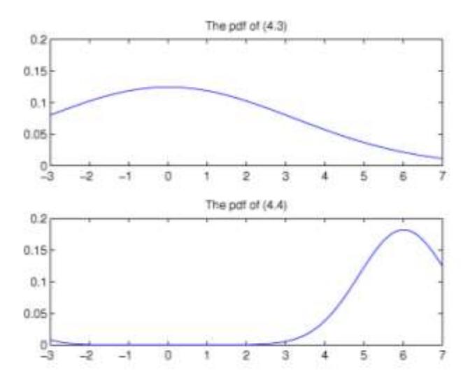
Figure 1 The pdf of \(Y_{n+1}\) conditional on \(Y_n = y_n\) (top) and the pdf of \(Y_{n+1}\) conditional on \(Y_n = y_n\) and \(|\widehat{\Theta} - 1| < \delta\) (bottom), M = 10.000.
we shall know that the vector \(Y = (Y_1, ..., Y_n)^T\) follows a multivariate normal distribution with mean vector \(\mu\) and the covariance matrix \(\Sigma\) i.e.
\[\text{[rumus tidak dapat ditampilkan dengan baik — lihat PDF asli]}\]
Now if we partition the mean vector \(\mu\) and the covariance matrix \(\Sigma\) such that
\[\mu = \begin{pmatrix} \mu_1 \\ \mu_2 \end{pmatrix}\] with sizes for \(\mu_1\) and \(\mu_2\) are \((n-1)\times 1\) and \(1\times 1\), respectively, and
\[\Sigma = \begin{pmatrix} \Sigma_{11} & \Sigma_{12} \\ \Sigma_{21} & \Sigma_{22} \end{pmatrix}\] with sizes
\[\begin{pmatrix} (n-1)\times(n-1) & (n-1)\times1 \\ 1\times(n-1) & 1\times1 \end{pmatrix}\]
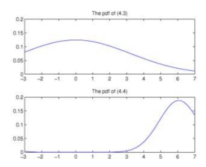
Figure 2 The pdf of \(Y_{n+1}\) conditional on \(Y_n=y_n\) (top) and the pdf of \(Y_{n+1}\) conditional on \(Y_n=y_n\) and \(|\widehat{\Theta}-1|<\mathcal{S}\) (bottom), M=50.000.
Then the distribution of \((Y_1,...,Y_{n-1})\) conditional on \(Y_n=y_n\) is multivariate normal with mean vector \(\mu\) and covariance matrix \(\Sigma\) ([9]), i.e.
\[(Y_1,...,Y_{n-1}|Y_n=y_n) \sim N(\mu, \Sigma)\] where the mean vector and the covariance matrix
\[\widetilde{\mu} = \mu_1 + \Sigma_{12} \Sigma_{22}^{-1} (y_n - \mu_2)\] \[\widetilde{\Sigma} = \Sigma_{11} - \Sigma_{12} \Sigma_{22}^{-1} \Sigma_{21}\]
Figures 1-3 show the pdf of \(Y_{n+1}\) conditional only on \(Y_n = y_n\) (top figure) and the pdf of \(Y_{n+1}\) conditional on \(Y_n = y_n\) and \(|\Theta| - 1| < \delta\) (bottom figure). We carry out n = 300 and M = 10,000,50000, and 100,000 simulation runs.
6 Discussion
The derivation of the asymptotic conditional coverage probability for a misspecified model requires a great deal more care than the derivation of the asymptotic conditional coverage probability for a properly specified model. Results similar to those of de Luna can be derived by defining the random variable \(\mathcal{E}_{n+1} = X_{n+1} - E(X_{n+1}|X_n,X_{n-1},\ldots)\) and noting that \(\mathcal{E}_{n+1}\) and \((X_n,X_{n-1},\ldots)\) are independent random vectors.
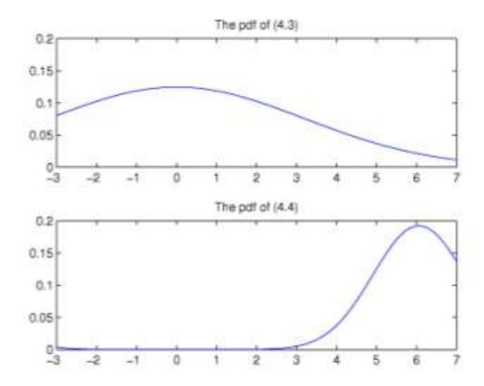
Figure 3 The pdf of \(Y_{n+1}\) conditional on \(Y_n=y_n\) (top) and the pdf of \(Y_{n+1}\) conditional on \(Y_n=y_n\) and \(|\widehat{\Theta}-1|<\delta\) (bottom), M=100.000.
\(X_{n+1} - E(X_{n+1}|X_n, X_{n-1},...)\) and noting that \(\mathcal{E}_{n+1}\) and \((X_n, X_{n-1},...)\) are independent random vectors.
Acknowledgement
I am grateful to Paul Kabaila for his valuable comments and suggestions to clarify many aspects on this paper.