1 Introduction

Methane as a greenhouse gas has a warming potential twenty three times greater than that of carbon dioxide, so removing it is important for environmental reasons. Furthermore, methane is a valuable energy source, so that an efficient conversion of methane to carbon dioxide would be doubly advantageous. This can be achieved by feeding oxygen and methane into a reactor. A catalyst is required to accelerate the conversion and normally preheating would be required to achieve optimal conversion conditions, however, by using the heat output from the reaction and appropriate cooling, preheating can be avoided and optimal chemical conversion conditions can be realized.

A concept successfully used in methane combustion is the catalytic reverse flow reactor (RFR). This concept was first discussed by Frank-Kamenetski [1] and was reviewed by Matros and Bunimovich [2]. An RFR is a packed-bed reactor in which the flow direction is periodically reversed totrap a hot zone within the reactor.

The common features of the combustion process in an RFR are usually the reaction-convection-diffusion equations with time-periodic coefficients and time-periodic boundary conditions. Garg, et al. [3] have observed that an adiabatic operation leads to periodic, period-1 symmetric states at which the temperature and concentrationprofiles at the beginning and end of a flowreversal period are mirror images.

Earlier studies [4-10] mostly focused on the determination of the steady state temperature profile within the reactor. The simulation of Gosiewski and Warmuzinsky [5] showed that the heat recovery by hot gas withdrawal from the reactor guaranteed more favorable symmetry of the half-cycle-temperature profile. For a cooled RFR, Khinast and Luss [8] observed that if reactor cooling was increased, the symmetric temperature profile became unstable and either a periodic asymmetric, a quasi-periodic or a chaotic state was obtained. Salomon, et al. [11] pointed out that the radial temperature gradient exists in both the inert and catalytic sections.

In this paper, we will discuss the steady state solution of the conversionof methane oxidation in an RFR in only one direction, from the left to the right end. We assume that the model is one-dimensional pseudo-homogeneous with small temperature variations and no heat loss. This leads to an equation in terms of the conversion variable only with an isothermal non linear reaction rate. For this case, the reaction can be considered to take place at a fixed temperature. Rescaling the variables, we obtain a dimensionless equation in which a small parameter is contained in the highest order of the equation,which leads to a singular perturbation problem. We solve the derived equation by using the matched asymptotic expansion method (see Holmes [12] orVerhulst [13]).

This paper is organized as follows. In Section 2, a mathematical model for steady state conversion of methane is described. The full equations are written in the Appendix. In Section 3, the asymptotic analysis using the singular

perturbation techniqueis presented to find the solution of steady state conversion. The conclusions are written in the last section.

2 Mathematical Model

In our study, we consider a cooled RFR described by a one-dimensional pseudo-homogeneous model that is taken from van Noorden [14], (see the detailed explanation in the Appendix). In the steady state, namely \(\chi_t = 0\), the resulting conversion equation is given by

\[K_5 \chi'' - K_6 \chi' + \widetilde{K}_7 (1 - \chi) = 0, \quad 0 \le x \le 1\] (1)

and boundary conditions are

\[K_5 \chi'(0) = K_6 \chi(0), \qquad \chi'(1) = 0,\] (2)

where \(\chi'' = \frac{d^2 \chi}{dx^2}\) and \(\chi' = \frac{d\chi}{dx}\). The values of the parameters are given in the Appendix.

Dividing both hand sides in (1) and (2) by \(\widetilde{K}_7\), we obtain

\[\varepsilon^3 \chi'' - \mu \varepsilon \chi' + (1 - \chi) = 0, \qquad 0 \le x \le 1 \tag{3}\]

\[\varepsilon^2 \chi'(0) = \mu \chi(0), \qquad \chi'(1) = 0 \tag{4}\] where \(\varepsilon^3=K_5\,/\,\tilde K_7\), and \(\mu=O(1)\). In the next section, we present an asymptotic solution for the system (3)-(4).

3 Asymptotic Solution

For \(\varepsilon \neq 0\), (3) has two linearly independent solutions. However for \(\varepsilon = 0\), (3) becomes a singular perturbation problem since we have a reduced order of the equation. To find the (outer) solution, we replace \(\chi(x)\) by \(y_0(x) + \varepsilon y_1(x) + \ldots\), and get for O(1) of (3)-(4) the following equations

\[1 - y_0 = 0, y_0(0) = 0, y_0'(1) = 0\] (5)

with the general solution

\[\chi_{outer} = y_0(x) = 1. \tag{6}\]

It is clear that (6) cannot fulfill the left boundary condition in (4). Thus, we end up with a boundary layer problem. To find the inner solution, we assume that there is a boundary layer at x = 0. Let

\[\xi = \frac{x}{\varepsilon^{\alpha}}.\tag{7}\]

Applying the chain rule, we have

\[\frac{d\chi}{dx} = \frac{d\chi}{d\xi} \frac{d\xi}{dx} = \frac{1}{\varepsilon^{\alpha}} \frac{d\chi}{d\xi}, \quad \frac{d^{2}\chi}{dx^{2}} = \frac{1}{\varepsilon^{2\alpha}} \frac{d\chi}{d\xi}.\] (8)

Subtitution of (7) and (8) in (3), yields

\[\varepsilon^{3-2\alpha} \frac{d^2 \chi}{d\xi^2} - \mu \varepsilon^{1-\alpha} \frac{d\chi}{d\xi} + (1-\chi) = 0 . \tag{9}\]

Let a solution \(\chi(\xi)\) of (9) be \(y_0(x) + \varepsilon y_1(x) + ...\)

\[\chi(\xi) = Y_0(\xi) + \varepsilon^{\gamma} Y_1(\xi) + \dots, \qquad \gamma > 0.\] (10)

Substituting the expansion in (10) into (9) we obtain

\[\varepsilon^{3-2\alpha} \frac{d^2}{d\xi^2} (Y_0(\xi) + ...) - \mu \varepsilon^{1-\alpha} \frac{d}{d\xi} (Y_0(\xi) + ...) + (1 - (Y_0(\xi) + ...)) = 0.\] (11)

The correct balancing in (11) occurs if \(3-2\alpha=1-\alpha\) or \(1-\alpha=0\), which implies that \(\alpha=2\) or \(\alpha=1\). In case \(\alpha=2\) we can write the O(1) boundary-layer equation

\[\frac{d^{2}Y_{0}}{d\xi^{2}} - \mu \frac{dY_{0}}{d\xi} = 0 \text{ for } 0 \le \xi < \infty \text{ and } Y_{0}(0) = \mu Y_{0}(0)\] (12)

The general solution of this problem is

\[Y_0(\xi) = Ce^{\mu\xi} + D, \tag{13}\] where C and D are arbitrary constants. The boundary condition in (12) gives D=0, thus (13) becomes

\[Y_0(\xi) = Ce^{\mu\xi}. \tag{14}\]

From (14), we recognize that for \(\xi \to \infty\), the solution tends to be unbounded, except for C=0. Thus for \(\alpha=2\), the inner solution \(Y_0(\xi)\) is trivial and it is not an asymptotic solution we need.

In the second case, \(\alpha = 1\), the boundary-layer Eq. (11) becomes

\[\varepsilon \frac{d^{2}}{d\xi^{2}} (Y_{0}(\xi) + ...) - \mu \frac{d}{d\xi} (Y_{0}(\xi) + ...) + (1 - (Y_{0}(\xi) + ...)) = 0,\] (15)

and the boundary condition leads to

\[\varepsilon(Y_0(0) + ...) = \mu(Y_0(0) + ...). \tag{16}\]

The O(1) equation is given by

\[\mu \frac{dY_0}{d\xi} + Y_0 = 1 ; Y_0(0) = 0, \tag{17}\] and the solution is

\[Y_0(\xi) = 1 - e^{-\xi/\mu} = 1 - e^{-x/(\mu\varepsilon)}.\] (18)

Note that from the O(1) equation for case \(\alpha = 1\) the matching process between the outer and the inner solutions automatically satisfied, i.e. \(Y_0(\infty) = y_0(0)\). Hence, the composite solution for O(1) is

\[\chi(x) = y_0(x) + Y_0(\xi) - y_0(1) = 1 - e^{-x/(\mu \varepsilon)}.\] (19)

For \(O(\varepsilon)\), from (3)-(4) we get the outer solution is \(y_1(x) = 0\) and from (15)-(16) the boundary layer equation is

\[\mu \frac{dY_1}{d\xi} + Y_1 = -\frac{1}{\mu^2} e^{-\xi/\mu} ; \mu Y_1(0) = Y_0(0),\] where the solution is given by

\[Y_{1}(\xi) = -\frac{1}{\mu^{3}} \xi e^{-\xi/\mu} + \frac{1}{\mu^{2}} e^{-\xi/\mu}. \tag{20}\]

Again, the matching process for \(O(\varepsilon)\) is automatically satisfied and then the composite solution is the inner solution \(Y_1(\xi)\), as in (20). So the asymptotic solution for our problem up to and including \(O(\varepsilon)\) is

\[\chi(x) = 1 - e^{-x/(\mu\varepsilon)} + \varepsilon \left( -\frac{1}{\mu^3} \xi e^{-\xi/\mu} + \frac{1}{\mu^2} e^{-\xi/\mu} \right) + \dots\] or

\[\chi(x) = 1 - e^{-x/(\mu\varepsilon)} - \frac{1}{\mu^3} x e^{-x/(\mu\varepsilon)} + \frac{\varepsilon}{\mu^2} e^{-x/(\mu\varepsilon)} + \dots\] (21)

In comparison, the exact general solution of (3) is

\[\chi(x) = 1 + Ae^{r_1x} + Be^{r_2x}. (22)\] with

\[r_1 = \frac{\mu + \sqrt{\mu^2 + 4\varepsilon}}{2\varepsilon^2}\] and \(r_2 = \frac{\mu - \sqrt{\mu^2 + 4\varepsilon}}{2\varepsilon^2}\).

If we expand \(\sqrt{\mu^2 + 4\varepsilon}\) at \(\varepsilon = 0\) until three terms and apply the boundary conditions (4), we get

\[A = \frac{\mu \left(\frac{\varepsilon}{\mu} - \frac{\varepsilon^2}{\mu^3}\right) e^{-\left(\frac{2}{\varepsilon\mu} + \frac{\mu}{\varepsilon^2}\right)}}{\left(\frac{\varepsilon}{\mu} - \frac{\varepsilon^2}{\mu^3}\right)^2 e^{-\left(\frac{2}{\varepsilon\mu} + \frac{\mu}{\varepsilon^2}\right)} - \left(\mu + \frac{\varepsilon}{\mu} - \frac{\varepsilon^2}{\mu^3}\right)^2 e^{-\frac{2}{\mu^3}}}\] and

\[B = \frac{\mu \left(\mu + \frac{\varepsilon}{\mu} - \frac{\varepsilon^2}{\mu^3}\right) e^{-\frac{2}{\mu^3}}}{\left(\frac{\varepsilon}{\mu} - \frac{\varepsilon^2}{\mu^3}\right)^2 e^{-\left(\frac{2}{\varepsilon\mu} + \frac{\mu}{\varepsilon^2}\right)} - \left(\mu + \frac{\varepsilon}{\mu} - \frac{\varepsilon^2}{\mu^3}\right)^2 e^{-\frac{2}{\mu^3}}}\]

The three term expansion of \(\sqrt{\mu^2 + 4\varepsilon}\) is considered since the roots \(r_1\) and \(r_2\) in

(22) contain a factor \(1/2\varepsilon^2\). For a small \(\varepsilon\), we note that \(e^{-\left(\frac{2}{\varepsilon\mu}+\frac{\mu}{\varepsilon^2}\right)}\) is smaller than any power of \(\varepsilon\) as \(\varepsilon\to 0\). Thus, for \(\varepsilon\to 0\) we get A tends to zero and B tends to -1. Hence, we can rewrite (22) as

\[\chi(x) = 1 - e^{\frac{\left(-\frac{2}{\mu}\varepsilon + \frac{2}{\mu^{3}}\varepsilon^{2} - \frac{4}{\mu^{5}}\varepsilon^{3} + \dots\right)x}{2\varepsilon^{2}}} + EST.\] \[= 1 - e^{\frac{x}{\mu\varepsilon}} e^{\left(\frac{1}{\mu^{3}} - \frac{2}{\mu^{5}}\varepsilon + \dots\right)x} + EST.\] (23)

where EST stands for exponentially small terms. In deriving the expansion (21), we expand \(e^{\left(\frac{1}{\mu^3} - \frac{2}{\mu^5}\varepsilon + ...\right)x}\) for x near the origin, so we get (23), as follows

\[\chi(x) = 1 - e^{-\frac{x}{\mu\varepsilon}} \left( 1 + \left( \frac{1}{\mu^3} - \frac{2}{\mu^5} \varepsilon + \dots \right) x + \dots \right).\]

\[=1-e^{-\frac{x}{\mu\varepsilon}}-\frac{x}{\mu^3}e^{-\frac{x}{\mu\varepsilon}}+\frac{2\varepsilon}{\mu^5}e^{-\frac{x}{\mu\varepsilon}}+\dots\] (24)

which is in agreement with (22), except for factor \(2\varepsilon/\mu^5\) in the fourth term.

Plots of the asymptotic solution and the exact and the numerical solution of (3)-(4) for \(\varepsilon = 0.05\) and \(\varepsilon = 0.005\) and \(\mu = 2\) are shown in Figure 1 and Figure 2. The numerical solutions of (3)-(4) are obtained by using the toolbox for boundary value problems in MATLAB.

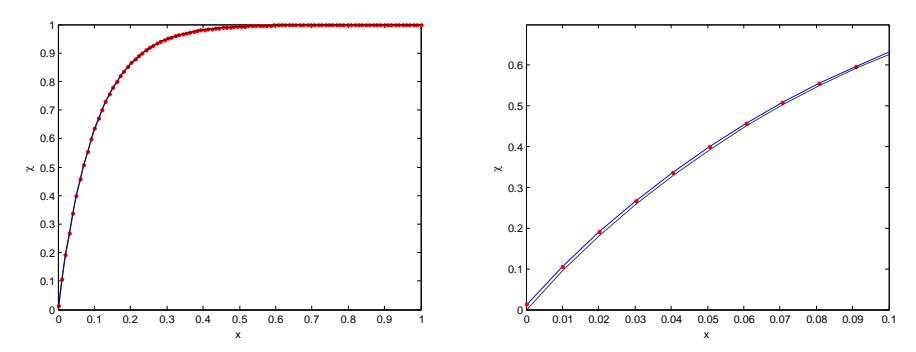
Figure 1 Left: Plot \(\chi\) of methane conversion as a function of position x, for \(\varepsilon = 0.05\) where the dashed line represents the exact solution and the solid line represents the asymptotic solution. The dotted symbol represents the numerical solution. Right: the zoom of \(\chi\) for a small window of x.

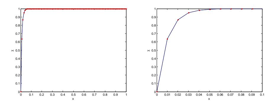
Figure 2 Left: Plot \(\chi\) of methane conversion as a function of position x, for \(\varepsilon = 0.005\) where the dashed line represents the exact solution and the solid line represents the asymptotic solution. The dotted symbol represents the numerical solution. Right: the zoom of \(\chi\) for a small window of x.

We observe that the results of the asymptotic solution and the numerical simulations hardly differ. The effect of reducing the magnitude of is to shorten the window of the rapid changes of the solution.

4 Conclusion

Based on available data, we constructed a singular perturbation problem for the steady state conversion of the methane oxidation process in a reverse flow reactor. The small parameter in our problem occurred both in front of the convective and diffusive terms in which the order of the diffusive term is higher than the convective one. Also, one of the boundary conditions had an order between the orderof those terms. Using the matched asymptotic expansion method and assuming that the boundary layer occurs at x 0, we solved the equation up to and including the first-order approximation. The present asymptotic solution was quite in agreement with the numerical solution and the exact solution.

Acknowledgements

The authors would like to thank the reviewers for their invaluable suggestions and corrections. This research was supported by Program Riset dan Inovasi KK ITB 2011 with grant no. 215/I.1.C01/PL/2011.