
1 Introduction
Crosshole tomography is a method to image the subsurface structure between two boreholes. The method is often employed for geotechnics and mineral exploration. In this study, crosshole tomography was used to image the depth of bedrock and ground water level.
The physical properties obtained from this method are seismic wave velocity and attenuation factor. Both physical properties can be used to determine depth of bedrock and ground water level.
This study was conducted on the main campus of Institut Teknologi Bandung (ITB), Indonesia. Two boreholes were used, LB1 and LB2, which were 19.8 meters apart (see Figure 1).
Figure 1 Location of two boreholes, LB1 and LB2.
2 Methodology
2.1 Ray Tracing
Ray tracing is a method to reconstruct rays from a source to a receiver. The algorithm used is the pseudo-bending method in which the algorithm is employed to minimize the travel time. This obeys Fermat's principle, which states that the wave propagates with minimum travel time (see Figure 2).
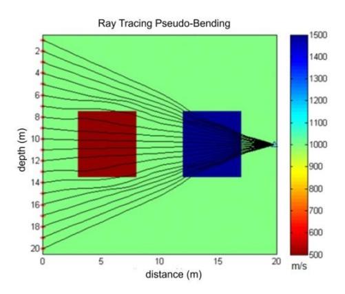
Figure 2 Test results of pseudo-bending ray tracing. Rays converge in the highvelocity anomaly and diverge in the low-velocity anomaly.
2.2 Travel Time Tomography
The travel time for direct wave T from a source i to a receiver j can be expressed using ray tracing as follows:
\[T_{ij} = \int_{source}^{receiver} u_{(x,y)} ds, \tag{1}\] where: \(u_{(x,y)}\) is the slowness (reciprocal of velocity), which is a function of position ds is the length of ray element.
Travel time \(t_{ij}\), can be written as follows:
\[t_{ij} = \tau_i + T_{ij}, \tag{2}\]
In this study, starting time \(\tau_i\) was 0 since we used active sources with known origin times. As a result, the arrival time was similar to the travel time. Ray path and slowness are parameters in the tomography inversion. However, both parameters are unknown.
The solution for a tomography inversion is a non-linear problem. The delay-time method can be used to solve iteratively the linearized approximation [1]. The norm and gradient are also utilized to obtain a block solution without a ray and smoothing model. The flow chart of the delay-time method can be seen in Figure 3.
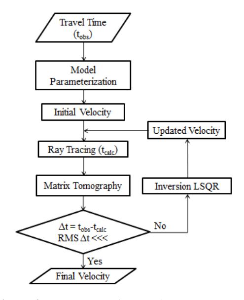
Figure 3 Flow chart of delay-time tomography.
The tomographic matrix equation can be written as follows:
\[\begin{pmatrix} A \\ \alpha I \\ \gamma G \end{pmatrix} \Delta m = \begin{pmatrix} \Delta t \\ 0 \\ 0 \end{pmatrix}, \tag{3}\]
\[\Delta t = t_{obs} - t_{calc}, \tag{4}\] where A is the length of the ray in each block, αI is norm damping and, γG is gradient damping. Δm is the slowness perturbation and Δt is the delay time.
\[m_{i+1} = m_i + \Delta m \tag{5}\]
Iterations stop when RMS becomes small and convergent.
2.3 Attenuation Tomography
The attenuation value of a medium is the inverse of the quality factor (Q), that is the ability of a medium to pass elastic wave energy [2]. The t* value is the attenuation parameter. In this study, t* was estimated from the equation,
\[t^* = \frac{t}{\varrho},\tag{6}\] where t is travel time and Q is the quality factor.
High dynamic range analysis of spectral waveforms was employed to calculate the t* value. An approximation by Eberhart-Phillips and Chadwick [3] was used to determine the velocity spectrum and t* inversion. Assuming an f 2 source model [4], velocity spectral amplitudes from source i to station j can be expressed as follows:
\[A_{ij}(f) = 2\pi f \Omega_0 \frac{f_c^2}{(f_c^2 + f^2)} \exp[-\pi f t_{ij}^*], \tag{7}\] where t*ij is the attenuation along the path. The three unknown parameters are corner frequency (fc), low frequency spectral level (Ω0), and attenuation operator (t*), which can be calculated using spectral-fitting.
t* is the travel time divided by the quality factor and can be written as the integration along the ray path from a source to a station, i.e. [5], [6], and [7].
\[t^* = \int_{raypat} \frac{1}{h} \frac{1}{Q_{(x,y)}V_{(x,y)}} ds, \tag{8}\]
4 shows a flow chart of the tomographic attenuation.
where velocity V is obtained from the delay-time tomography inversion. Figure
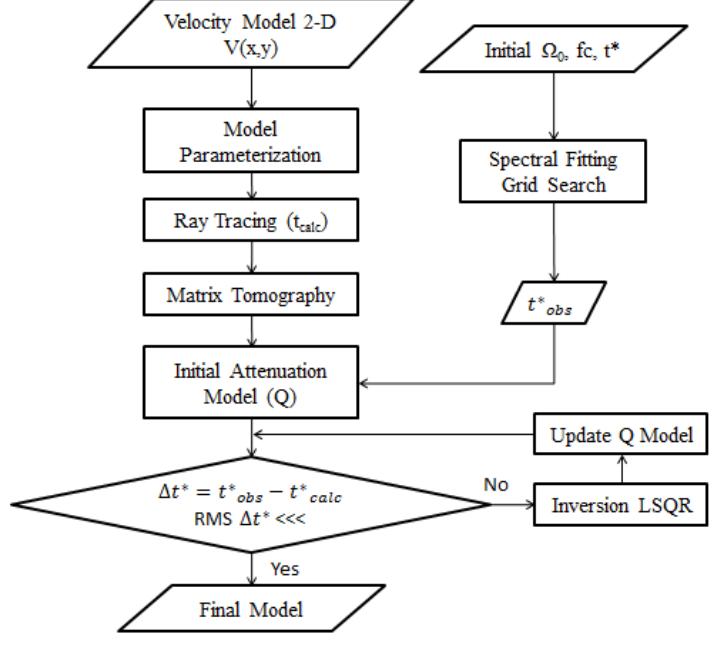
Figure 4 Flow chart of tomographic attenuation.
3 Data Acquisition and Processing
3.1 Equipment
In this study a sparker was used as the source of seismic P-waves generated by an impulse generator (IPG 1005). Seismic waves were recorded by a string of hydrophones, type-III with 12 channels. A sample rate of 50 µs was used with a record length of 51.2 ms and 200 μs with a length of 204.8 ms.
3.2 Borehole Scheme
The distance between the two boreholes was 19.80 meters. The depth of the first borehole (LB1) was more than 39 meters, while the second borehole (LB2) was 19 meters deep. LB1 was used for the sources and LB2 was used for the receivers. The sources were exploded from depths of 17 to 39 meters at 1 meter intervals. The receivers were located at depths of 1 meter to 19 meters with 1 meter intervals (see Figure 5).
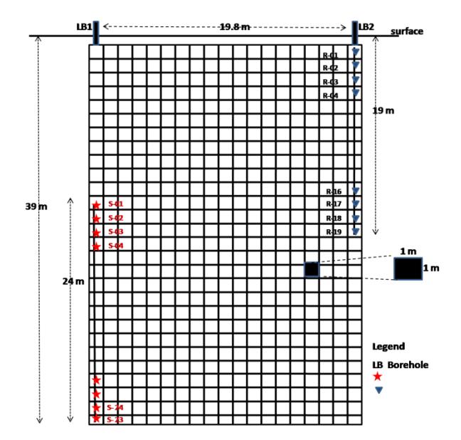
Figure 5 Borehole scheme. There are 23 source positions and 19 receiver positions. Model parameterization uses a grid with size of 1x1 m2 .
3.3 Data Preparation
Field records were arranged according to common sources. Figure 6 shows the common source data after noise correction.
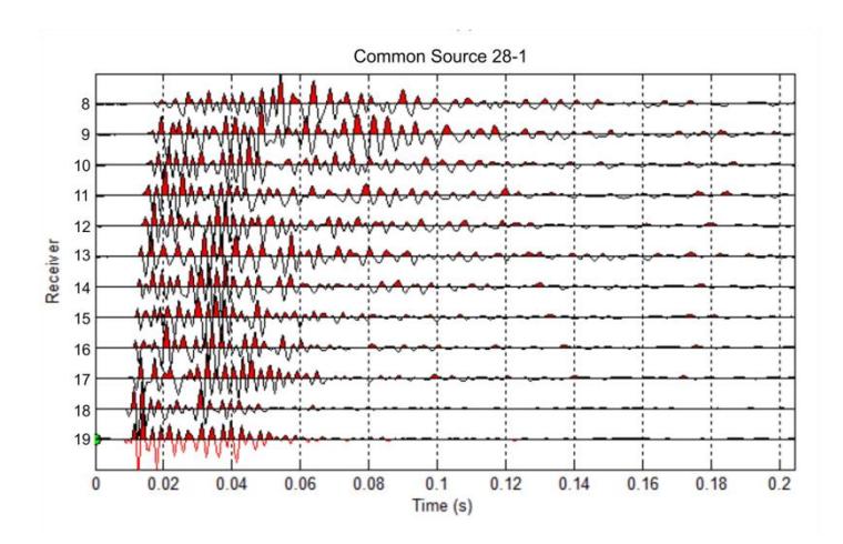
Figure 6 Common Source 28-1 filtered with tube wave. The tube wave propagates along a fluid-filled well. Therefore it was affected by responses of geophones as noises. Later on, we filtered the waveform data to reduce the influence of noise.
3.4 Picking First Break
For picking the first break of the P-waves, the Akaike Information Criterion (AIC) method was used. Subsequently, the results were organized into catalog data (see Figure 7).
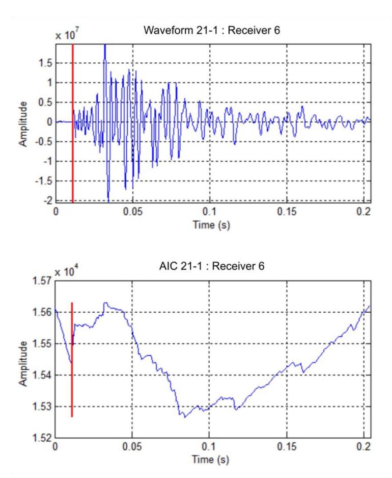
Figure 7 Waveform and picking of first break (top) and AIC (bottom). The AIC method, which is based on the variance data, can distinguish the arrival time clearly.
4 Results
4.1 Model Parameterization
Model parameterization used homogeneous blocks with a size of 1x1 m2 with 20 blocks horizontally and 39 blocks vertically.
4.2 Initial Velocity
The initial velocity was obtained from a 1-D tomography with the gradient velocity as a function of depth that can be expressed as follows:
\[V(z) = V_0 + kz (9)\] where V(z) is the velocity at depth z, V0 is the first layer velocity, and k is the velocity factor gradient.
In the study, V0 = 500 m/s and the velocity gradient k = 50.6 m/s. Results from the 1-D tomography are shown in Figure 8, which was used as the initial model.
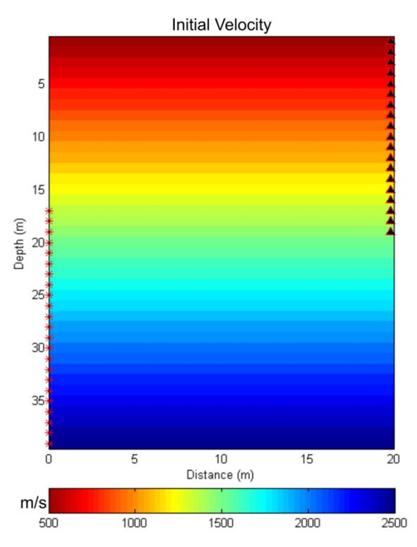
Figure 8 Initial 1-D velocity model used for 2-D tomographic inversion.
4.3 Checkerboard Resolution Test
The Checkerboard Resolution Test (CRT) is forward modelling employed to test the reliability of an inversion method. The results of this test show that there was good resolution when a cell was passed by many ray paths (see Figure 9).
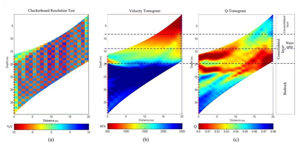
Figure 9 (a) Inversion results of checkerboard resolution test. (b) Inversion results for the velocity. (c) Inversion results for Q-tomography. Both the velocity and Q inversions show that there is an unconsolidated layer (down to 8 meters), a consolidated layer (from 8 meters down to 20 meters), and bedrock ( > 20 meters).
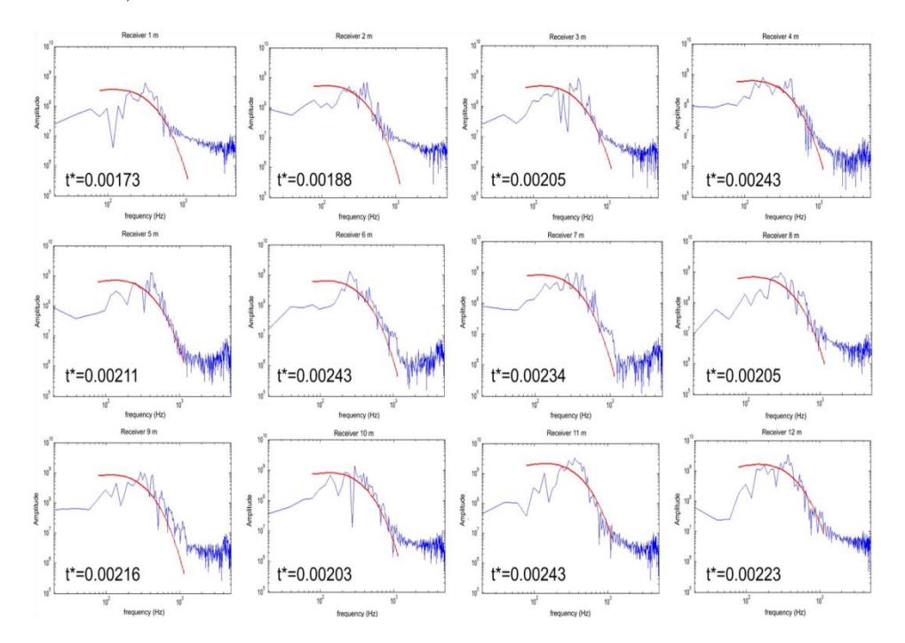
Figure 10 Result of spectral fitting using a grid search for common source 29- 1. Corner frequency (fc) of the source was estimated to be 462 Hz.
5 Conclusions
The tomographic inversion results for both the velocity and attenuation show that there are three rock layers: an unconsolidated layer (down to depth of 8 meters), a consolidated layer (from 8 to 20 meters in depth), and bedrock ( > 20 meters in depth).
It is estimated that the water table is at a depth of 14 meters.
The results of the Q tomographic inversion can be used to identify a water saturated zone that corresponds to a low-quality factor.