
1 Introduction
Several successful applications of the EnKF in reservoir estimation have been reported. Lorentzen, et al. [1] applied the EnKF to a PUNQ-S3 reservoir model. The parameters were permeability and porosity, and the measurements consisted of bottom-hole pressure, water cuts and gas-oil ratios. Yu [2] used the EnKF for the optimization of reservoir models. Mantilla, et al. [3] used the
EnKF for updating geologic models for water coning control. Gu and Oliver [4] reported the use of the EnKF for history matching.
The EnKF is a sequential estimation method that can be used to estimate reservoir parameters. It combines modeling and data measurement. Reservoir parameters play an important role in characterizing a reservoir for improving its performance. The parameters discussed in this study were permeability and porosity. The EnKF was applied to estimate both parameters.
The purpose of this paper is to discuss the applicability of the EnKF methodology for estimating reservoir parameters. The flow in the reservoir was modeled as two interacting wells through the diffusivity equation for pressure. The Laplace transform was used to obtain an analytical solution of the diffusivity equation. A simulation study showed that the proposed method can be used successfully to estimate the reservoir parameters using well-pressure observations.
2 Methodology
Consider a linear flow between two interacting wells separated by distance \(\ell\). The reservoir is assumed homogeneous, i.e. the reservoir has a single value of permeability and porosity. The diffusivity equation was used to describe the fluid flow distribution in porous media. An analytical solution was obtained using the Laplace transform. Two cases were considered: (i) constant pressure and (ii) constant rate. The diffusivity equation was written in the form of pressure P(x, t) which depends on the distance from the injection well and time t.
\[\frac{\partial^2 P}{\partial x^2} = \frac{1}{n} \frac{\partial P}{\partial t}, \quad 0 < x < \ell \tag{1}\] where \(\eta = .00264\frac{k}{\varphi\mu c}\) is the hydraulic coefficient, k is the permeability, \(\varphi\) is the porosity, \(\mu\) is the viscosity, c is the total compressibility, x is the distance from the injection well and \(\ell\) is the distance between the injection well and the production well. The initial and boundary conditions were:
(i) constant pressure: \[P(x,0) = P_0, P(0,t) = P_0, P(\ell,t) = P_1, P_1 > P_0\],
(ii) constant rate: \[P(x,0) = Cx\], \(\frac{\partial P}{\partial x}(0,t) = C\), \(P(\ell,t) = P_1\).
The solutions for both cases are [5]
(i) \[P(x,t) = P_0 + V \sum_{i=0}^{\infty} \left\{ erfc \frac{(2i+1)\ell - x}{2\sqrt{\eta t}} - erfc \frac{(2i+1)\ell + x}{2\sqrt{\eta t}} \right\}\] (2)
and
(ii) \[P(x,t) = Cx + V \sum_{i=0}^{\infty} (-1)^{n} \left\{ erfc \frac{(2i+1)\ell - x}{2\sqrt{\eta t}} - erfc \frac{(2i+1)\ell + x}{2\sqrt{\eta t}} \right\}\] (3)
where \(V = P(\ell, t) - P_0\).
Data assimilation refers to a method of information integration provided by feeding measurements into estimates of state. The Kalman filter is one of the most well-known data assimilation methods (Wikle and Berliner [6]). The model produces a forecast at the observation time. This forecast is used as a prior in the Kalman filter process. By weighting the bias of observation and forecast, the filter makes an adjustment to the estimate of state. Consider the evolution of states \(X_{\tau}\) and observations \(Y_{\tau}\).
\[\begin{cases} X_{t} = FX_{t-1} + W_{t} & W_{t} \sim N(0, Q) \\ Y_{t} = HX_{t} + V_{t} & V_{t} \sim N(0, R) \end{cases}\] \[(4)\] where Q is model error covariance, R is the observation error covariance, F is the model operator, and H is the observation operator. Y, are noisy observations of a subset of X. One cycle of data updating consists of a forecast (prior) and an update (posterior). The forecast relies on the state estimate at t-1 to produce an optimal forecast at t. In updating, the measurement information from t is used to refine the forecast to obtain a more accurate state estimate. Statistics of the forecast are represented by forecast state X<sub>t</sub> and forecast error covariance \(P_t^f = E((X_t^f - X_t)(X_t^f - X_t)^T)\) and update state \(X_t^u\) and update error covariance \(P_t^u = E((X_t^u - X_t)(X_t^u - X_t)^T)\). As the most well-known estimation method, the Kalman filter provides a recursive state estimation at each observation time. Each cycle consists of a forecast and an update. An initial guess is known, \((X_0^u, P_0^u)\), \(P_0^u = E((X_0^u - X_0)(X_0^u - X_0)^T)\), and \(X_0^u - X_0\) is uncorrelated to \(W_t\) and \(V_t\). For each cycle t, the algorithm consists of: forecast \(X_t^f = FX_{t-1}^u\), \(E((X_{t-1}^u - X_{t-1}^u).W_t^T) = 0\), \(P_t^f = FP_{t-1}^u F^T + Q\), update: \(X_t^u = X_t^f + K(Y_t - HX_t^f)\), \(K = P_t^f H^T (HP_t^f H^T + R_t)^{-1}\), \(P_t^u = (I - KH)P_t^f\). The Ensemble Kalman filter was proposed in order to solve a problem related to the implementation of the
Kalman filter in nonlinear systems. The EnKF is a Monte Carlo simulation of state and observation. The distribution of states is represented by a collection of states called an ensemble. The estimates for the state given by the EnKF converges (in probability) to the results given by the Kalman filter. The distribution of states estimation is represented by the realizations of state known the forecast ensemble \(\{X_{t,i}^f, i=1,2,...,n\}\) and update ensemble \(\left\{X_{t,i}^u, i=1,2,\ldots,n\right\}\). The forecast error covariance \(P_t^f\) and update error are approximated \(\hat{P}_{k,n}^{f} = \frac{1}{n} \sum_{t=1}^{n} \left( \left( X_{t,i}^{f} - \overline{X}_{t}^{f} \right) \left( X_{t,i}^{f} - \overline{X}_{t}^{f} \right)^{t} \right), \quad \overline{X}_{k}^{f} = \frac{1}{n} \sum_{t=1}^{n} X_{t,i}^{f}, \quad \hat{P}_{t,n}^{f} = \frac{1}{n} \sum_{t=1}^{n} \left( \left( X_{t,i}^{u} - \overline{X}_{t}^{u} \right) \left( X_{t,i}^{u} - \overline{X}_{t}^{u} \right)^{T} \right),\)\(\overline{X}_t^u = \frac{1}{n} \sum_{t,i}^n X_{t,i}^u\). The initial sample is represented by \(\left\{X_{0,i}^u = X_0^u + W_{0,i}, \right\}\)\(\text{[rumus tidak dapat ditampilkan dengan baik — lihat PDF asli]}\)\(W_{t,i} \sim N(0,Q), i=1,...,n\), \(\overline{X}_t^f = \frac{1}{n} \sum_{t,i}^n X_{t,i}^f\). The Kalman gain is computed as \(\hat{K} = \hat{P}_t^f H^T (H \hat{P}_t^f H + R)^{-1}\). The update is given by \(X_{t,i}^u = X_{t,i}^f + \hat{K} (Y_{t,i} - H X_{t,i}^f)\), \(Y_{t,i} = Y_t + V_{t,i}, V_{t,i} \sim N(0,R)\). A basis for the validity of the EnKF is the asymptotic convergence (Tan [7], Li and Xiu [8]), \(\bar{X}_{t,n}^f = \frac{1}{n} \sum_{t,i}^n X_{t,i}^f \rightarrow_p X_t^f\)\(\hat{P}_{t,n}^{f} = \frac{1}{n} \sum_{t=1}^{n} P_{t,i}^{f} \rightarrow_{p} P_{t}^{f}, \text{ for all } t=1,2,.... \ \overline{X}_{t,n}^{u} = \frac{1}{n} \sum_{t=1}^{n} X_{t,i}^{u} \rightarrow_{p} X_{t}^{u} \ \hat{P}_{k,n}^{u} = \frac{1}{n} \sum_{t=1}^{n} P_{t,i}^{u} \rightarrow_{p} P_{t}^{u}\)\(\{X_{i,i}^{f}, i=1,2,...,n\}\) is the forecast ensemble, \(\{X_{i,i}^{u}, i=1,2,...,n\}\) is the update ensemble, \(P_t^f\) is the forecast error covariance matrix, \(P_t^u\) is the update error \(\text{[rumus tidak dapat ditampilkan dengan baik — lihat PDF asli]}\)\(\frac{1}{n}\sum_{t=0}^{n}\left(X_{t,i}^{u}-\overline{X}_{t}^{u}\right)\left(X_{t,i}^{u}-\overline{X}_{t}^{u}\right)^{T}, \ \overline{X}_{t}^{u}=\frac{1}{n}\sum_{t=0}^{n}X_{t,i}^{u} \ \text{are sample covariance matrices.}\)
The autoregressive of order 1, AR(1), is the basic model in time series modeling. Consider a state space representation for AR(1) with ensemble size n = 1: \(X_t = X_{t-1} + W_t\), \(W_t \sim N\left(0, Q = 10^{-4}\right)\), \(Y_t = X_t + V_t\), \(V_t \sim N\left(0, R = 10^{-1}\right)\) with initial estimate: \(X_0^u = 0\), \(P_0^u = 1000\), measurement \(Y_1 = .9\). Calculations for the first iteration yield: forecast \(X_1^f = X_0^u = 0\), \(P_1^f = P_0^u + Q = 1000.0001\), update \(K_1 = 1000.0001(1000.0001 + .1)^{-1} = .9999\), \(X_1^u = X_1^f + K\left(Y_1 - X_1^f\right) = 0 + .9999(.9 - 0)\)
= .8999, \(P_1^u = (1 - K_1)P_1^f = (1 - .9999)1000.0001 = .1\). The update step has brought the initial value 0 to the true value 1. The second iteration yields: forecast \(X_2^f = X_1^u = .8999\), \(P_2^f = P_1^u + Q = .1 + .0001 = .1001\), update: \(K_2 = .1001\) \((.1001 + .1)^{-1} = .5002\), \(X_2^u = .8999 + .5002(.8 - .8999) = .8499\), \(P_2^f = (1 - .5002)\) .1001 = .05. A summary of the iterations is shown in Table 1. Synthetic data were used to see if the filter behaved as it should. The filter converged to what it thinks is the true value X = 1.
Table 1 Data assimilation for static model, ensemble size n = 1, state and observation error variance \(Q = 10^{-4}\), \(R = 10^{-1}\). The estimate stabilized after the 4<sup>th</sup> iteration, even though the measurements were between .9 and 1.2.
| t | Forecast | Update | ||||
|---|---|---|---|---|---|---|
| t | \(X_t^f\) | \(\mathbf{P}_{\mathrm{t}}^{\mathrm{f}}\) | \(\mathbf{Y}_{t}\) | \(\mathbf{K}_{t}\) | \(\mathbf{X}_{\mathrm{t}}^{\mathrm{u}}\) | \(\mathbf{P}_{t}^{\mathrm{u}}\) |
| 0 | 0 | 1000 | ||||
| 1 | 0 | 1000.0001 | .9 | .9999 | .8999 | .1 |
| 2 | .8999 | .1001 | .8 | .5002 | .8499 | .05 |
| 3 | .8499 | .0501 | 1.1 | .3339 | .9334 | .0334 |
| 4 | .9334 | .0335 | 1.0 | .2509 | .9501 | .0251 |
| 5 | .9501 | .0252 | .95 | .2012 | .9501 | .0201 |
| 6 | .9501 | .0202 | 1.05 | .1682 | .9669 | .0168 |
| 7 | .9669 | .0169 | 1.2 | .1447 | 1.0006 | .0145 |
In standard data assimilation methodology, a linear model between the state and the observations is assumed. For interacting wells, this assumption does not hold. To be able to use the EnKF in this situation, the state has to be extended to include the observations. This construction allows to consider cases in which the observations are a nonlinear function of the parameters. This approach is known as extended state. In this study, the extended state becomes \(X_t = \left(k_t - P(k_t, x, t)\right)^T\). A state space representation for a nonlinear model f is given by \(X_t = f\left(X_{t-1}\right) + \epsilon_t^m\), \(Y_t = HX_t + \epsilon_t^{obs}\). For the case of permeability, the state space representation is given by
\[X_{t} = \begin{pmatrix} k_{t} \\ P_{t} \end{pmatrix} = \begin{pmatrix} k_{t-1} \\ P(x, t, k_{t}) \end{pmatrix} + \begin{pmatrix} 0 \\ \varepsilon_{t}^{m} \end{pmatrix}, Y_{t} = HX_{t} + \varepsilon_{t}^{obs}, H = \begin{pmatrix} 0 & 1 \end{pmatrix}.\]
Before any observations (well pressure) are history matched, a sample of size n is generated at t=0 from prior distributions. Only the model parameters in the state are generated. Using prior information, the model is advanced to the first observation. This is called the forecast step, where the pressure and permeability are predicted. Once the forecast step is completed, the samples of permeability and pressure are updated, based on the observed pressure. The updating process is performed on the entire state; permeability and pressure are updated at the same time. If the relationship between parameter and observation is linear, the results are exact; if it is nonlinear they are approximate. Once the state is updated, the forecast is repeated and another update is performed. The process is repeated until all observations are history matched. The initial parameter distribution represents the expert estimate of the parameters. The EnKF requires the specification of variance for errors in the model and for errors in the observations. In case of a small error variance for the observations, one assumes that the observations are fairly accurate.
3 Results and Discussion
A twin experiment is an experiment in which the data are simulated using a model. In this study, a twin experiment was used to show the applicability of the method. Using a twin experiment, one can show the convergence of the proposed method. Figure 1 shows the results for permeability of Case i (constant pressure). The simulation was set up for experiment time T = 100, x = 10050, n = 30, m = 100, \(\sigma_k = 8\), \(\sigma_p = .8\), \(k_{\text{true}} = 22\). The initial sample was generated from \(k \sim N(17.8^2)\), \(P \sim N(1..8^2)\). The observed pressure successfully updated the permeability estimate. A pressure history match was attained after a number of updating steps. The permeability estimate converged to the true permeability value after updating 14 times. Figure 2 presents the results of the porosity estimation from the constant-pressure model (Case i). The simulation was set up for experiment time T = 100, x = 50, n = 30, m = 100, \(\phi_{true} = 30\%\), \(\sigma_{_0} = .5, \sigma_{_P} = .5\). The pressure successfully updated the porosity estimate. A pressure history match was attained after a number of updating steps. The porosity update converged to the true porosity after updating 4 times. The porosity of the reservoir rocks may vary from 5% to 30%. Porosity is of primary importance in reservoir engineering because it is a measure of the space available for the storage of oil fluids within a reservoir rock.
Figures 3 and 4 show the results of the reservoir simulation. The oil production and water production are shown in Figure 3. The oil reservoir bottom-hole pressure showed a declining pattern, as shown in Figure 3. Figure 4 shows the results of the permeability estimation using the EnKF procedure. There was a good match between the observed pressure and its prediction. The sequential permeability estimation showed a convergence to the true value of the reservoir permeability (200 mD). The results show that the proposed method can be used successfully to estimate the reservoir parameters using reservoir simulation data.
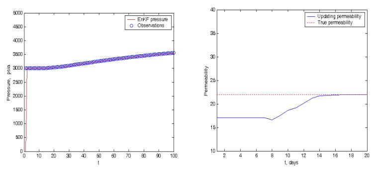
Figure 1 Forecast and update of permeability and history match of pressure for Case i (constant pressure). True permeability was 25 mD.
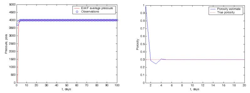
Figure 2 Forecast and update of porosity and history match of pressure for Case i (constant pressure). True porosity was 30%.
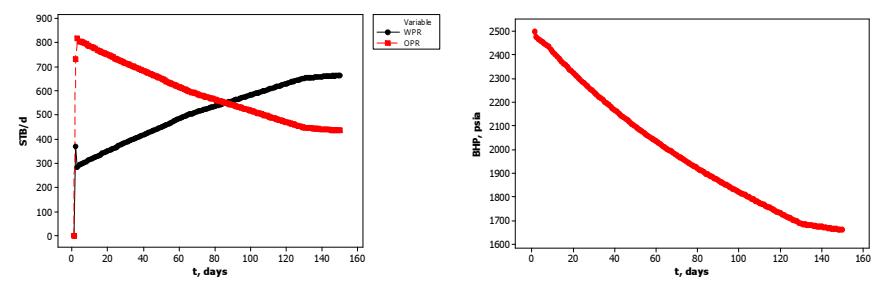
Figure 3 Oil production (STB/d), water production (STB/d), and bottom-hole pressure (BHP, psia) of production well from reservoir simulator ECLIPSE in a two injection-production system. Reservoir parameters were: porosity 40%, permeability 200 mD, total production 1100 STB/d, water injection rate 500 STB/d, well distance 1697 ft. The well pressure showed a declining pattern.
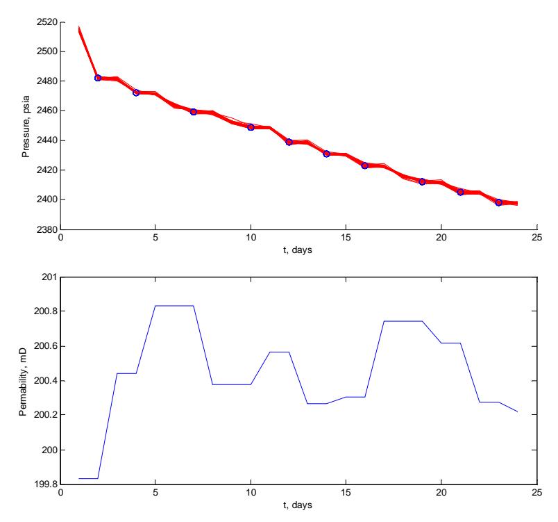
Figure 4 Permeability estimation using reservoir simulator data. The figure shows a good match with the well-production data. The sequential permeability estimate showed convergence to the real permeability value of 200 mD.
4 Conclusions
The EnKF is a promising method for optimizing reservoir models, updating reservoir simulation models, updating geologic models, etc. However, a lot of work has to be done in this area. This paper investigated the applicability of this method for estimating the permeability and porosity in two interacting wells. A diffusivity equation was used to describe the fluid flow in the system. Using the Laplace transform, an analytical solution was established. A state space model was constructed and an EnKF algorithm was established. A simulation study for cases of constant pressure and constant rate showed that the method can be used successfully to estimate the reservoir properties (permeability and porosity).
Nomenclature
c = compressibility, 1 psi−
C = constant for constant-rate initial condition
erfc = complementary error function
k = permeability, mD K = Kalman gain
\(\hat{K}\) = sample Kalman gain
\(\ell\) = distance between injection well and production well, m
m = number of observations
n = ensemble size
\(N(\mu, \sigma^2)\) = normal distribution with mean \(\mu\) and variance \(\sigma^2\)
P(x, t)= pressure at distance x from the injector at time t, psi
\(P_t^i\) = forecast error covariance at time t
\(\hat{P}_{t,n}^f\) = sample forecast error covariance at time t
\(P_t^u\) = update error covariance at time t
\(\boldsymbol{\hat{P}}^{u}_{t,n}~=~\text{sample}\) update error covariance at time t
Q = model error covariance, mD<sup>2</sup> R = observation error covariance
t = time, hours
T = experiment time, hours
x = distance from injection well, m X<sub>t</sub> = state (unobservable) at time t, mD
\(X_{\star}^{f}\) = forecast state at time t, mD
\(X_{t,i}^{f}\) = forecast ensemble at time t, mD
\(X^{u}_{\cdot}\) = update state at time t
\(X_{t,i}^{u}\) = update ensemble at time t
\(Y_t\) = observations at time t, psi
\(V = P(\ell,t) - P(0,t)\) = pressure difference between injection and production
well at time t, psi
\(\eta\) = hydraulic coefficient
φ = porosity, %μ = viscosity, cp
\(\sigma_{\rm p}\) = standard deviation for pressure, psi
\(\sigma_k\) = standard deviation for permeability, mD
Acknowledgements
This work is funded by ITB research program contract No. 426/I.1.c.01/PL/2012. We would like to thank the editors and the reviewer for improving the quality of our paper.