
1 Introduction
Controlled-source audio-frequency magnetotellurics (CSAMT) is a high-resolution electromagnetic sounding technique that uses a grounded electric dipole as the source of artificial signals. CSAMT is a variant of magnetotellurics (MT); the main difference with conventional MT is the use of artificial signals. CSAMT was originally introduced by Goldstein and Strangway [1] to solve signal stability problems in the MT method. Artificial sources produce a stable signal, allowing high-precision data acquisition and faster time measurement than natural sources.
There are many works on controlled-source electromagnetic modeling for 2D electromagnetic modeling with 3D finite source, such as Unsworth, et al. [2], and Mitsuhata [3]. Li and Key [4] developed a 2D marine controlled-source electromagnetic modeling method using an adaptive finite element algorithm. Streich [5] used the finite-difference frequency domain (FDFD) scheme for 3D modeling of marine controlled-source electromagnetic modeling. To avoid effects by the presence of an artificial source, CSAMT data are usually taken at a distance of 3-5 skin depth from the source using the plane wave approach [6]. Yamashita, et al. [7] and Bartel and Jacobson [8] proposed a source effect correction and used plane wave approach to interpret the corrected data. Nearfield corrections have received serious attention since they are based on a homogeneous earth model and have validity under question in complicated environments [9]. As shown by Routh and Oldenburg, the use of MT inversion for the interpretation of CSAMT data can lead to unexpected results [9]. Hence they introduced a full solution CSAMT inversion to avoid this problem and stated the importance of full solution CSAMT to interpret CSAMT data [9].
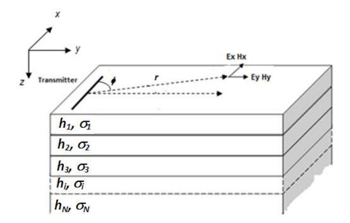
Figure 1 Vector CSAMT field setup over a 1D layered earth.
There are several types of CSAMT data measurement, based on the number of components of measurement, which can be classified as tensor, vector, or scalar measurement [10]. Vector CSAMT is defined as a four- or five-component measurement, which consists of Ex, Ey, Hx, Hyand optionally Hz , excited by a single source polarization [10]. Scalar CSAMT only uses a two-component measurement (Ex–Hy measurement, or the so-called xy configuration; and Ey–Hx measurement, or the so-called yx configuration). Usually, conventional 1D CSAMT surveys use scalar CSAMT, which has low operational cost and a high production speed of data acquisition [10]. Since the earth is complex, a more sophisticated configuration could be set up in order to obtain better data, such as a vector and tensor CSAMT configuration. In this study, vector and scalar CSAMT were used to interpret full solution CSAMT data. We have developed a forward modeling of vector and scalar 1D CSAMT based on the full CSAMT solution. The performance of vector CSAMT compared to scalar CSAMT was tested by applying the developed modeling to the smoothness-constrained Occam inversion developed by Constable, et al. [11].
2 The EM Field Generated by CSAMT
1D CSAMT data can be considered as electromagnetic field excitation generated by a horizontal electric dipole (HED) over a layered earth. Calculation of the electric and magnetic fields generated by HED has been widely performed and can be found in many works [12-14].
A vector CSAMT configuration usually consists of two electrodes and two magnetic antennas, as shown in Figure 1. Suppose the layered-earth model consists of n layers with each layer having conductivity value \(\sigma_i\) and thickness \(h_i\) (Figure 1). A horizontal electric dipole located on the surface is placed parallel to the x axis. A receiver is located at distance r from the dipole. The direction of the receiver is calculated from the dipole center with an angle \(\phi\), the angle formed between the x-axis and the direction of the receiver. The components of the electric and magnetic fields generated by electric dipole excitation sources in cylindrical coordinates measured at the surface expressed as follows [12,13]:
\[H_R = \frac{-Idx}{2\pi r} \sin \varphi \left[ \int_0^\infty \frac{m}{m+\hat{Y}_1} J_1(mr) dm + r \int_0^\infty \hat{Y}_1 \frac{m}{m+\hat{Y}_1} J_0(mr) dm \right]\] (1)
\[H_{\varphi} = \frac{Idx}{2\pi r} \cos \varphi \left[ \int_{0}^{\infty} \frac{m}{m + \hat{Y}_{1}} J_{1}(mr) dm \right]\] (2)
\[E_{R} = \frac{Idx}{2\pi r} \cos \varphi \left\{ \frac{i\omega\mu}{r} \int_{0}^{\infty} \frac{1}{m+\hat{Y}_{1}} J_{1}(mr) dm - \rho_{1} \int_{0}^{\infty} \hat{Y}_{1}^{*} m J_{0}(mr) dm + \frac{\rho_{1}}{r} \int_{0}^{\infty} \hat{Y}_{1}^{*} J_{1}(mr) dm \right\}\] \[\left\{ + \frac{\rho_{1}}{r} \int_{0}^{\infty} \hat{Y}_{1}^{*} J_{1}(mr) dm \right\}\] \[(3)\]
\[E_{\varphi} = \frac{Idx}{2\pi r} \sin \varphi \begin{cases} \frac{\rho_{1}}{r} \int_{0}^{\infty} \hat{Y}_{2} J_{1}(mr) dm - i\omega \mu \int_{0}^{\infty} \frac{m}{m + \hat{Y}_{1}} J_{0}(mr) dm \\ + \frac{i\omega \mu}{r} \int_{0}^{\infty} \frac{1}{m + \hat{Y}_{1}} J_{1}(mr) dm \end{cases}\] \[(4)\]
\(\hat{Y}_1\) and \(\hat{Y}_2\) are the admittances of the lower half-space, which can be expressed recursively as [12,13]:
\[\hat{Y}_{1} = Y_{1} \frac{\hat{Y}_{2} + Y_{1} \tanh(u_{1}h_{1})}{Y_{2} + \hat{Y}_{1} \tanh(u_{1}h_{1})}\] (5)
\[\hat{Y}_{1}^{*} = Y_{1} \frac{\hat{Y}_{2}^{*} + Y_{1}^{*} \left(\frac{\sigma_{2}}{\sigma_{1}}\right) \tanh\left(u_{1}h_{1}\right)}{Y_{2}^{*} \left(\frac{\sigma_{2}}{\sigma_{1}}\right) + \hat{Y}_{1}^{*} \tanh\left(u_{1}h_{1}\right)}\] (6)
\[\hat{Y}_{n} = Y_{n} \frac{\hat{Y}_{n+1} + Y \tanh(u_{n} h_{n})}{Y_{n+1} + \hat{Y}_{n} \tanh(u_{n} h_{n})}\] (7)
\[\hat{Y}_{n}^{*} = Y_{n} \frac{\hat{Y}_{n+1}^{*} + Y_{n}^{*} \left(\frac{\sigma_{n+1}}{\sigma_{n}}\right) \tanh\left(u_{n}h_{n}\right)}{Y_{n+1}^{*} \left(\frac{\sigma_{n+1}}{\sigma_{n}}\right) + \hat{Y}_{n}^{*} \tanh\left(u_{n}h_{n}\right)}\] \[(8)\] with
\[Y_{n} = Y_{n}^{*} = u_{n}\] \[u_{n} = \left(k_{x}^{2} + k_{y}^{2} - k_{n}^{2}\right)^{1/2} = \left(\lambda^{2} - k_{n}^{2}\right)^{1/2}\] \[k_{n}^{2} = \omega^{2} \mu_{n} \varepsilon_{n} - i\omega \mu_{n} \sigma_{n}\]
Eqs. (1)–(4) are usually called full solution CSAMT equations, since they describe the field behavior in all zones of radiation (i.e. near field zone, transition field zone and far field zone). The field components in Cartesian coordinates \(E_x\), \(E_y\), \(H_x\) and \(H_y\) are calculated using the following transformations [12]:
\[E_{x} = E_{r} \cos \varphi - E_{\varphi} \sin \varphi\] \[E_{y} = E_{r} \sin \varphi + E_{\varphi} \cos \varphi\] \[H_{x} = H_{r} \cos \varphi - H_{\varphi} \sin \varphi\] \[H_{y} = H_{r} \sin \varphi + E_{\varphi} \cos \varphi\] \[(9)\]
In geophysical prospecting, the electromagnetic responses are generally expressed in apparent resistivity and phase of impedance. Apparent resistivity are expressed as follows [10,15]:
\[\rho_{xy} = \frac{1}{\omega u} |Z_{xy}|^2, \rho_{yx} = \frac{1}{\omega u} |Z_{yx}|^2\] (10)
With the \(Z_{xy}\) and \(Z_{yx}\) components are the impedance for expressed as
\[Z_{xy} = \frac{E_x}{H_y}, Z_{yx} = \frac{E_y}{H_x}\] (11)
Eq. (10) is known as Cagniard's apparent resistivity equation. The other important component is the phase of impedance which can be written as
\[\varphi_{xy} = \arctan\left(\frac{im(Z_{xy})}{re(Z_{xy})}\right),\] \[\varphi_{yx} = \arctan\left(\frac{im(Z_{yx})}{re(Z_{yx})}\right)\] (12)
In Eq. (12) \(\phi\) is the phase of the impedance, which has a value of 45° in a homogeneous medium. The index xy and yx shows the measurement configuration as shown in Figure 1.
For the computation of infinite integrals containing Bessel functions of order 0 and 1 that appear in the equation of the EM field components, the fast Hankel transform algorithm developed by Anderson [16,17] is used. The Hankel transform of order n = 0.1 is defined by [16,17]:
\[f(r) = \int_{0}^{\infty} K(\lambda) J_{n}(r\lambda) d\lambda , r > 0\] (13)
\(J_n\) is the Bessel function of the first kind and order n.
In this study, a code for full solution 1D CSAMT based on Eqs. (1)–(4) has been developed. This code calculates the electromagnetic responses (i.e. electric and magnetic fields in radial and azimuthal components) of HED, transforms the components into Cartesian coordinates and obtains the CSAMT responses in the form of apparent resistivity and phase of impedance. A flow chart of the code is shown in Figure 2.
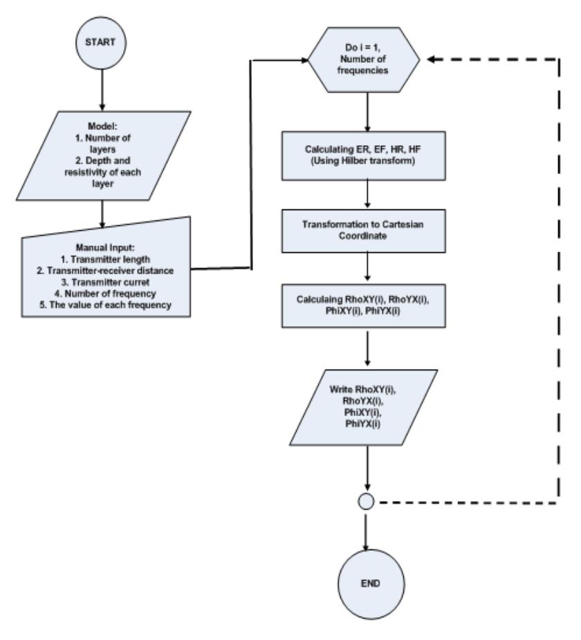
Figure 2 Flow chart of full solution 1D CSAMT modeling.
3 Occam's Smoothness-Constrained Inversion
The inversion scheme used in this study is the Occam inversion developed by Constable, et al. [11]. Occam's inversion produces a smooth model and fits the model to data sets with some tolerance, although the model may not be the best model for the data. A non-linear inversion problem can be formulated as a minimization of the regularization model space matrix that qualifies the misfit of a certain value δ in data space. In a mathematical expression, the inversion problem can be formulated as [11,18,19]:
\[\min \|L_m\| \quad \text{and} \quad \|\mathbf{WG}(\mathbf{m}) - \mathbf{Wd}\| \le \delta \tag{14}\] where L is a finite-difference approximation of differential of first and second order and
\[\mathbf{W} = diag\left\{\frac{1}{\sigma_1}, \frac{1}{\sigma_2}, \frac{1}{\sigma_3}, \dots \frac{1}{\sigma_N}\right\}\] (15)
Eq. (15) states W as a diagonal matrix with a value inversely proportional to the standard deviation of the i-th data, which is usually used as a weighting function. Thus, the misfit can be expressed as [11,18]:
\[\chi^{2} = \sum_{i=1}^{N} \frac{\left(d_{i} - G_{i}(\mathbf{m})\right)^{2}}{\sigma_{i}^{2}}\] (16)
If there is a mode lm, using Taylor's theorem we can develop an approximation as follows:
\[\mathbf{G}(\mathbf{m} + \Delta \mathbf{m}) \approx \mathbf{G}(\mathbf{m}) + \mathbf{J}(\mathbf{m}) \delta \mathbf{m}\] (17)
J(m) is the Jacobian matrix.
By using this approximation, the damped least squares Eq. (14) can be written as:
\[\min \|\mathbf{W}(\mathbf{G}(\mathbf{m}) + \mathbf{J}(\mathbf{m})\Delta\mathbf{m} - \mathbf{d})\|^{2} + \alpha^{2} \|\mathbf{L}(\mathbf{m} + \Delta\mathbf{m})\|^{2}\] (18)
To simplify the formulation of the problem, this approximation is usually written with variable \((m+\Delta m)\):
\[\min \|\mathbf{WJ}(\mathbf{m})(\mathbf{m} + \Delta \mathbf{m}) - (\mathbf{Wd} - \mathbf{WG}(\mathbf{m}) + \mathbf{WJ}(\mathbf{m})\mathbf{m})\|^{2} + \alpha^{2} \|\mathbf{L}(\mathbf{m} + \Delta \mathbf{m})\|\](19)
The solution of Eq. (17) can be written as follows [11,18,19]:
\[\mathbf{m} + \Delta \mathbf{m} = (\mathbf{WJ}(\mathbf{m})^T \mathbf{WJ}(\mathbf{m}) + \alpha^2 \mathbf{L}^T \mathbf{L})^{-1} * \mathbf{WJ}(\mathbf{m})^T \mathbf{W} \hat{\mathbf{d}}(\mathbf{m})\](20)
This method is similar to the Gauss-Newton method used in the damped least squares problem. The iteration can be used to solve Eq. (14) for some value \(\alpha\) and then pick the highest \(\alpha\) value for which the model is appropriate with constrained data \(\|\mathbf{WG}(\mathbf{m}) - \mathbf{Wd}\| \le \delta\) [18,19].
4 Interpretation of Synthetic Data
The models used to generate the synthetic data were as follows:
- 1. A three-layer earth with one conductive layer trapped between two resistive layers (typical for geothermal sites).
- 2. A three-layer earth with one thin resistive layer trapped between two conductive layers (typical for hydrocarbon sites).
- 3. The models are shown in Figure 3. To interpret the synthetic data, the following steps were taken:
- 4. The responses were simulated using the developed forward modeling code. The synthetic responses were in the form of apparent resistivity and phase of impedance in the xy and yx configurations.
- 5. Next, the synthetic responses were inverted using both vector and scalar CSAMT. The xy and yx responses were inverted simultaneously for the vector CSAMT, while the scalar CSAMT inverted the responses separately for both xy and yx.
- 6. The models generated by the inversion in Step (2) were then compared to synthetic models. The compatibility of the inversion models with the synthetic models was expressed as relative RMS error.
- 7. The models resulted from the inversion were then used for forward modeling. The results were inversion responses that were compared to synthetic responses. The compatibility of both responses (i.e. inversion and synthetic responses) was expressed as relative RMS error.
The earth in this modeling was parameterized as a layered earth with 40 layers, each layer having an exponentially increasing thickness, with a depth as proposed by Routh and Oldenburg [9]. The modeling was simulated on a dipole source-receiver distance of \(R_X = 2000\) meter and \(R_Y = 500\) meter, as shown in Figure 2. At this distance, the source effect is still dominant that the plane wave assumption is invalid and hence the full solution interpretation should be applied. The dipole length is 1000 meters with a current strength of 1 ampere. The model's responses were calculated 16 audio frequencies with a value of \(2^N\) Hz and N is an integer with a value ranging from -2 to 13 (the range of frequencies from 0.25 Hz to 8192 Hz).
The compatibility of the inversion models and responses with the synthetic models and responses were calculated using relative RMS error:
\[RMS = \sqrt{\frac{1}{N} \sum_{i=1}^{N} \left\{ \frac{(d_i - t_i)}{t_i} \right\}^2 \times 100\%}\] (21)
N is the number of data, \(d_i\) the i-th inversed model or data, and \(t_i\) the i-th synthetic model or data. The relative RMS error between the synthetic and the inverted models and responses for model 1 and model 2 are described in Table 1 and 2.
The first model (Figure 3(ii)) is a typical geothermal site with a conductive layer between two resistive layers. The obtained inversion model showed fairly good compatibility with the synthetic models for both vector and scalar CSAMT, as shown in Figure 4. From Table 1 it is clear that the model generated by vector CSAMT is better than the one generated by scalar CSAMT. Figure 5 shows good compatibility between the inversion and the synthetic responses for apparent resistivity and phase of impedance (Table 1). Nevertheless, the response generated by vector CSAMT shows good results compared to scalar CSAMT, with a relative RMS error lower than 0.2%. The results demonstrate the importance of vector CSAMT inversion to obtain more accurate data interpretation.
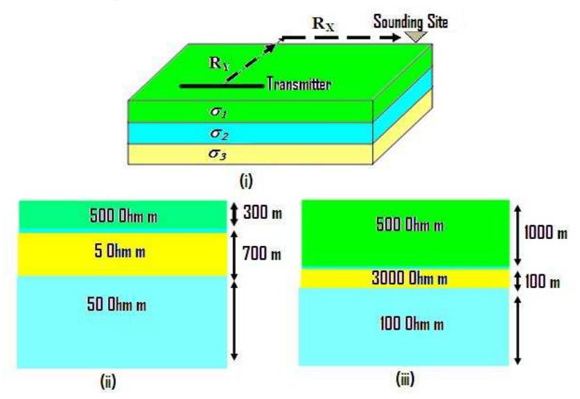
Figure 3 (i) The field setup used for the modeling. RYand RXshows the distance of transmitter-receiver (sounding site) in Cartesian coordinates. (ii) Synthetic model 1, with a conductive layer buried within a relatively resistive layer. (iii) Synthetic model 2, with a thin resistive layer buried within a relatively conductive layer.
The second model (Figure 3(iii)) was a layered earth typical for hydrocarbon exploration, in which a very thin resistive layer (100 meters) lies on a depth of 1000 meters between relatively conductive layers. As in the first model, the model resulted from vector CSAMT inversion had good compatibility with the synthetic data relative to scalar CSAMT (Figure 6). Table 2 shows the quantitative aspect of the inversion models and responses, where the relative RMS error of vector CSAMT was in the range of 6%, while for scalar CSAMT
it was about 20%. Once again, the results show the importance of vector
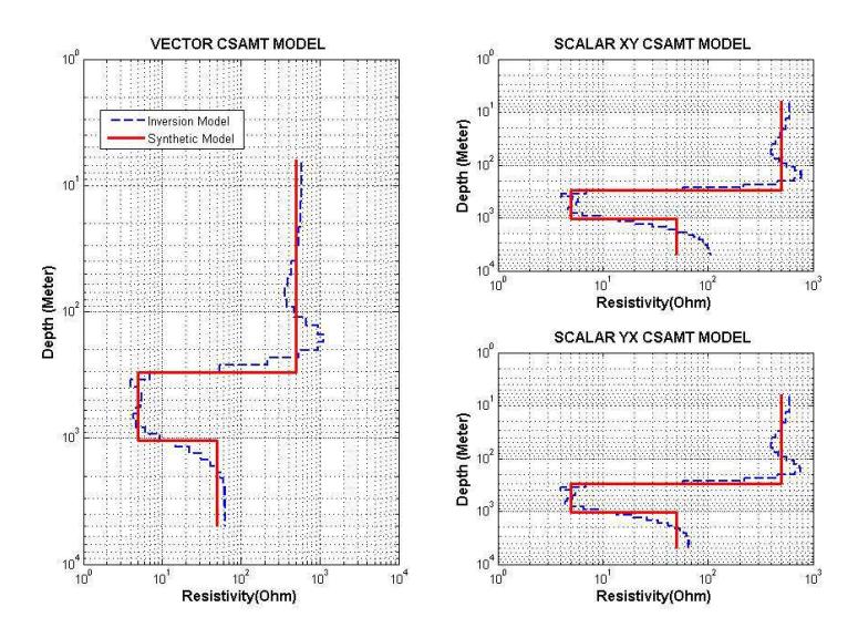
Figure 4 Comparison of synthetic model 1 to inversion models generated by vector and scalar CSAMT.

Figure 5 Comparison of synthetic responses of model 1 with the inversion responses, generated by vector and scalar CSAMT.
.
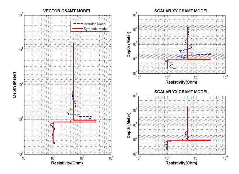
Figure 6 Comparison of synthetic model 2 to inversion models generated by vector and scalar CSAMT.
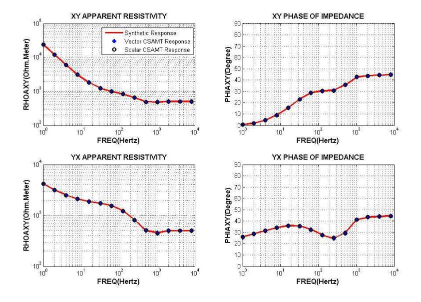
Figure 7 Comparison of synthetic responses of model 2 with the inversion responses, generated by vector and scalar CSAMT.
CSAMT interpretation. The synthetic and the inversion responses are shown in Figure 7. According to Table 2, the synthetic and inversion responses have excellent compatibility with the highest error: only in the range of 1%. However, the model generated by vector CSAMT is more accurate than the models generated by scalar CSAMT.
In general, from synthetic models both the vector and the scalar CSAMT responses had a very good match with the synthetic response. Nevertheless, the model generated by vector CSAMT had a better fit than the models generated by scalar CSMAT. Thus, vector CSAMT interpretation is needed to obtain more accurate models.
Table 1 Relative RMS error of CSAMT inversion compared to synthetic model and responses for model 1.
| Relative RMS Error | VECTOR CSAMT(%) | SCALAR CSAMTXY (%) | SCALAR CSAMTYX (%) | |
|---|---|---|---|---|
| Model | 4.21 | 13.35 | 13.17 | |
| Apparent Resistivity | 0.12 | 0.45 | 1.25 | |
| Phase of Impedance | 0.077 | 0.21 | 0.84 | |
Table 2 Relative RMS error of CSAMT inversion compared to synthetic model and responses for model 2.
| Relative RMS Error | VECTOR CSAMT (%) | SCALAR CSAMT XY (%) | SCALAR CSAMT YX (%) |
|---|---|---|---|
| Model | 6.37 | 21.60 | 19.68 |
| Apparent Resistivity | 0.11 | 0.049 | 1.33 |
| Phase of Impedance | 0.093 | 0.14 | 1.13 |
5 Application to Field Data
The performance of the developed vector CSAMT code was tested using field data. The inversion of two geothermal sites was performed using both vector and scalar CSAMT. The RX and RY distances (i.e. the distance of transmitterreceiver separation, described in Cartesian axes, as shown in Figure 2) were 3354 meters and 1064 meters respectively for site T01, and 2978 meters and 2312 meters respectively for site T02. The data used for inversion are apparent resistivity for both the xy and yx configuration. The compatibility of the field data with the inversion responses is shown in Table 3.
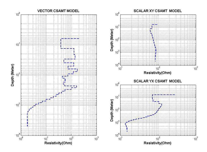
Figure 8 The model generated by vector and scalar CSAMT inversion for the data of site T01.
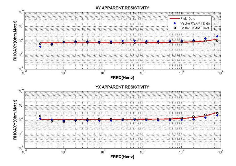
Figure 9 Comparison of field data of site T01 with the inversion responses generated by vector and scalar CSAMT.
Figure 8 shows the models generated from inversion of both vector and scalar CSAMT for site T01. The models generated by vector CSAMT show a relatively more complex structure than those generated by scalar CSAMT. Scalar xy shows a relatively homogeneous layer, while scalar yx describes a simple layered earth. This result clearly shows the importance of interpretation using the vector CSAMT, where the scalar CSAMT could lead to different interpretation. Figure 9 shows a comparison of field data with the inversion data for both vector and scalar CSAMT. From Table 3 it can be seen that the relative RMS error of the vector CSAMT responses was higher than that of the scalar xy CSAMT (0.96% compared to 0.56%), but both responses had approximately the same error level (about 1 %).
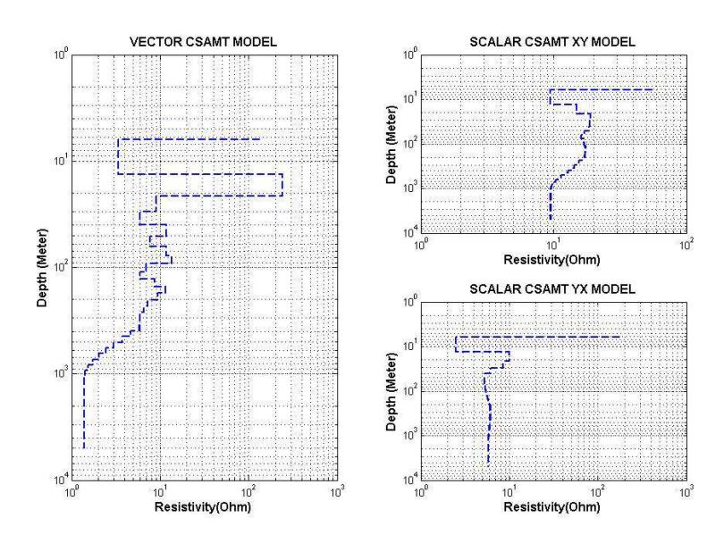
Figure 10 The model generated by vector and scalar CSAMT inversion for the data of site T02.
The models generated from the data of site T02 are shown in Figure 10. As before, the vector CSAMT led to a complex structure, while the scalar CSAMT led to a relatively simple structure. The compatibility of the field data with the inversion responses is shown in Figure 11. It is clear from Figure 11 and Table 3 that the responses from the vector CSAMT had a relatively high error compared to those of scalar xy CSAMT. For site T02, the relative RMS error for both vector and scalar yx was about 3%, while for scalar xy it was below 2%. However, in general the error was still relatively low and can be assumed compatible. Nevertheless, the models generated by vector and scalar CSAMT
led to different structures. This shows the necessity to use the vector CSAMT. In real earth the data seem to be affected by 3D conductivity structures [9]. This circumstance leads to a more complicated interpretation, because the 1D layered earth assumption cannot be made. A more sophisticated configuration, such as tensor CSAMT, may be used to give a better interpretation of the earth's complexities.
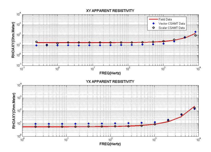
Figure 11 Comparison of field data of site T02 with the inversion responses generated by vector and scalar CSAMT.
Table 3 Relative RMS error of CSAMT inversion compared to synthetic model and responses for model 2.
| SITES | VECTOR CSAMT (%) | SCALAR CSAMT XY (%) | SCALAR CSAMT YX (%) |
|---|---|---|---|
| T01 | 0.96 | 0.56 | 1.03 |
| T02 | 3.38 | 1.77 | 3.53 |
6 Conclusion
In this paper a forward modeling of full solution 1D CSAMT has been developed to invert CSAMT data. The performance of the forward modeling has been tested using two synthetic models which characterized two geological features: (i) a conductive layer buried between resistive layers, as usually found in geothermal sites; and (ii) a thin resistive layer buried between conductive
layers, as typically found in hydrocarbon exploration. The inversion has been taken for both models using vector and scalar CSAMT. The results showed that the models generated by vector CSAMT were more compatible with the synthetic models than those generated by conventional scalar CSAMT. The relative RMS error for the synthetic data inversion shows the importance of vector CSAMT interpretation. The relatively small error of the responses as shown in Table 1 and 2 does not guarantee a perfect match between the synthetic and the inversion models. The tables clearly show the superiority of vector CSAMT to interpret CSAMT data, since the scalar CSAMT provides less structure information.
The performance of the developed modeling was tested using field data of two geothermal sites, with a relatively close transmitter-receiver distance. Application to the field data showed complex structure models generated by vector CSAMT, while scalar CSAMT led to more simple models. The big difference between both measurements simply confirms the superiority of vector CSAMT over conventional scalar CSAMT. The results confirm the lack of information carried by scalar CSAMT to describe the conductivity structures of the earth. Nevertheless, a more sophisticated measurement (i.e. tensor CSAMT measurement) should be applied to obtain more information about conductivity structures.
Acknowledgements
The authors would like to express their gratitude to LPPM-ITB for funding this research through the Riset KK ITB 2009.