
1 Introduction
Coastal aquifers often provide the water supply for domestic, industrial, or agricultural water demands. Although the economics of groundwater development in many regions of the world are cost-effective, sustained overdraft distorts the natural recharge-discharge equilibrium. The principal environmental impact associated with groundwater overdraft is saltwater intrusion, arguably one of the most significant water quality problems. Moreover, over-reliance on groundwater in coastal aquifers in many countries has also produced declining water levels, well yields, a reduction in groundwater storage, and land subsidence.
Saltwater intrusion is a global problem. For example, saltwater intrusion is a major problem in the Yun Lin basin in southwestern Taiwan. This basin has been the second largest agricultural producing region of Taiwan. However, the increasing demand to expand agricultural production has produced a pattern of declining well yields and land subsidence in the southwestern portion of the basin, the Peikang region. Agricultural production has been severely reduced in this area.
Saltwater intrusion also continues to impact Jakarta, Indonesia. As shown in Figure 1, the Jakarta groundwater system is a complex, multi-aquifer system – a system that is hydraulically interdependent. Withdrawals from one of the aquifers influence water levels and salinity in the adjacent aquifers.
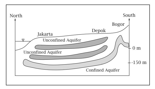
Figure 1 Jakarta Groundwater System [1].
Over 80% of Jakarta's daily water demand is supplied by groundwater. The overdevelopment of groundwater has reduced well discharges and water levels and increased salinity intrusion. Water levels in shallow unconfined aquifers are below sea level over a large area of the coastal plain during the dry season. The average cone of depression is approximately 5 meters below sea level. Piezometric heads in the basin's leaky aquifers have also decreased to more than 20 m below sea level in the coastal areas of Jakarta. The annual decline in the piezometric head averages between 2 and 7 m/year.
In the United States, saltwater intrusion is a serious problem both on the east and west coasts. Freshwater aquifers on the east coast of the United States supply more than 30 million people. Saltwater intrusion on the east coast has been documented throughout the coastal zone from Maine to Florida [2].
On the west coast of the United States, the Oxnard groundwater basin, located 60 miles northwest of Los Angeles, has documented intrusion problems since at least the 1930s [3]. It became a serious issue in the 1950s. Approximately 23 mi2 of the upper portion of the groundwater system have been degraded by saltwater.
The underlying issue associated with all of these problems is a lack of understanding of how the groundwater system responds (in space and time) to variations in natural recharge and discharge, and groundwater pumping and artificial recharge.
The objective of this paper is to present an overview of how optimization models are used for the control of saltwater intrusion. In contrast to simulation analysis, which is essentially a trial-and-error approach in resolving management issues, optimization identifies the "best" or optimal pumping and recharge strategies. The strategies or policies are consistent with the stipulated economic, hydrologic, or environmental objectives and constraints of the management or planning problem. Specifically, the paper presents (a) an optimal control model for basin-wide management of saltwater intrusion, and (b) a linked simulation-optimization algorithm for the control of saltwater intrusion.
2 The Seawater Intrusion Problem
Over the past three decades, two methodologies have been used for the simulation of saltwater intrusion. The first approach assumes that a sharp interface exists between fresh water and salt water. The second is based on the advection-dispersion equation; saltwater intrusion is described as a densitydependent transport process. These models are described and developed in [4- 7].
2.1 Response Equations
The development of optimization models for the control and management of saltwater intrusion is based on equations describing the saltwater intrusion process. The sharp-interface and the density-dependent models are both described by coupled systems of nonlinear partial differential equations [6,7]. The transformation or approximation of these equations via numerical methods produces the response equations of the coastal aquifer system. The response equations are those equations that explicitly relate the state variables of the problem, the freshwater and saltwater heads, the pressure field, or the mass fractions, and the groundwater controls – the magnitude, location, and duration of groundwater pumping and/or artificial recharge.
Historically, the approximation of the saltwater intrusion equations has been approached using boundary integral, finite difference, and a variety of finite element procedures. Representative boundary integral studies include Liu, et al. [8] and Taigbenu, et al. [9]. Finite element methods have been used to develop both two-dimensional vertically averaged models and fully three-dimensional
models. Finite element studies include Huyakorn, et al. [10], Voss and Souza [11], Pinder and Gray [12], and Hayler [13]. Finite difference models include Mercer, et al. [14], Essaid [6], Pinder and Cooper [15] (finite differences and the method of characteristics) and Kipp [7].
The hydraulic and water response equations of the coastal aquifer system have the same general form for either the finite difference or finite element numerical transformation of the spatial derivatives. Assuming that the boundary conditions for the problem have been specified completely, the response equations for a sharp-interface coastal aquifer are [1],
\[\frac{d\Phi}{dt} = \mathbf{f}(\mathbf{h}_f^{\ell}, \mathbf{h}_s^{\ell}, \mathbf{Q}_l^{\ell}), \ \ell \in \Gamma_{\ell}\] (1)
\[\Phi(\mathbf{x},0) = \Phi_0 \tag{2}\] where is a vector containing the freshwater and saltwater heads, is a vectorvalued function of the finite difference or finite element (transformed) equation, is the set of initial conditions, denotes the aquifer layer, and Q is a vector of possible pumping and artificial recharge rates, e.g. pumping pattern, the control variables of the management problem.
In density-dependent transport, the response equations are [7],
\[A\frac{d\theta}{dt} + B\theta + \mathbf{f}(\mathbf{Q}) = \mathbf{0} \tag{3}\]
\[\theta(\mathbf{x},0) = \theta_0 \tag{4}\] where is a vector containing the pressure field and mass fraction , and is the set of initial conditions. The coefficient matrices, A and B, incorporate the system's parameters and discretization. The f contains the boundary conditions, sources and the control variables, Q.
3 The Optimal Control Model
The control or management of saltwater intrusion is readily formulated as a problem in optimal control. The management model maximizes or minimizes benefit, cost, or state variable functionals while satisfying pumping or recharge targets, well capacity limitations, and possible bounds on the state variables, e.g. freshwater and saltwater heads, pressures, or mass fractions. The control variables of the problem determine the magnitude of pumping or artificial recharge in any planning period. The control variables are required to satisfy the equations of motion of the system, the response equations of the aquifer system. The control problem may be expressed as:
\[\min_{\mathbf{p}(t)} J = \int_{t_0}^{t_f} e^{-\alpha t} L(\mathbf{x}(t), \mathbf{p}(t), t) dt\] (5)
subject to
\[G(\mathbf{x}(t), \mathbf{p}(t)) \le \bar{G}(\mathbf{x}(t), \mathbf{p}(t))\] (6)
\[\mathbf{x}(t) \in R^n \tag{7}\]
\[\mathbf{p}(t) \in R^m \tag{8}\] where is the objective functional, is time, is the beginning of the planning horizon, is the end of the planning horizon, is the discount factor when economic rather than physical surrogate objectives are used in the optimization model. is the state vector, and is the control vector defining the pumping and/or artificial recharge occurring in the aquifer system. Eq. (6) are general constraints dependent on both the state and the control variables. Eq. (7) limits the state variable variation in the aquifer, for example to minimize excessive drawdowns or well interference effects from occurring in the basin, or to limit salinity intrusion. Eq. (8) are control constraints that restrict the magnitude of groundwater pumping and recharge.
The final components of the control model is the initial conditions and the equations of motion of the control problem, Eqs. (1-2) and Eqs. (3-4).
4 Algorithms
Previous studies have demonstrated several possible algorithms for the solution of field-scale seawater intrusion control problems. Several of these algorithms are discussed below.
4.1 Control Solution-Imbedding Method
An obvious solution algorithm is the direct solution of the optimal control problem. However, the application of the maximum principle produces a nonlinear multi-point boundary value problem [16]. Typically these types of problem can be solved using variants of quasilinearization and/or invariant imbedding.
4.1.1 Optimization Problem
A more direct solution of the control problem involves the transformation of the problem into a discrete-time mathematical optimization problem [17]. The discrete-time optimization problem, which is similar to Eqs. (5)-(8), can be expressed as
\[\min_{\mathbf{p}_t} J = \sum_{t=1}^{N} \frac{L_t(\mathbf{x_t}, \mathbf{p_t}, t) \, \Delta t}{(1+\rho)^t} \tag{9}\]
subject to
\[G(\mathbf{x}_t, \mathbf{p}_t, t) \le \bar{G}(\mathbf{x}_t, \mathbf{p}_t, t), \quad t = 1, 2, \dots, N\] (10)
\[\mathbf{x}_t \in R^n \tag{11}\]
\[\mathbf{p}_t \in R^m \tag{12}\] where now the state and control variables are written for every over the entire planning horizon, and is the discount factor.
The equations of motion for the sharp-interface model can be expressed via the finite difference approximations of the time derivatives, or from Eqs. (1) and (2),
\[\frac{d\Phi}{dt} \approx \frac{\Phi^k - \Phi^{k-1}}{\delta \tau} = \mathbf{f}(\mathbf{h}_f^{\ell,\tau}, \mathbf{h}_s^{\ell,\tau}, \mathbf{Q}_l^{\ell,t}), \ \ell \in \Gamma_\ell, \ \forall \tau \in \Delta t\] (13)
\[\Phi(\mathbf{x},0) = \Phi_0 \tag{14}\]
Where is the length of the finite difference time step, and the equations are written for all finite difference time steps over a planning period, .
In the density-dependent case, Eqs. (3) and (4) can be approximated as,
\[\frac{d\theta}{dt} \approx \frac{\theta^k - \theta^{k-1}}{\delta \tau} = R\theta^k + \mathbf{g}(\mathbf{Q^t}), \ \forall \tau \in \Delta t\] (15)
\[\theta(\mathbf{x},0) = \theta_0 \tag{16}\] where and
The control problem is a nonlinear, nonconvex optimization problem. The nonconvexity of the problem implies that there are potentially many locally optimal solutions to the planning or management problem.
The transformation of the optimal control problem into an optimization model is essentially a variant of the imbedding approach of groundwater management [18]. In this approach, the response equations are written explicitly as a set of auxiliary constraints for the planning model. The advantage of this approach is that the optimization simultaneously identifies the state and control variables, e.g. the simulation and optimization problem have been effectively combined into one problem. Moreover, the state variable tradeoffs are determined directly from the solution of the optimization problem. Examples of this approach are presented in Willis and Liu [19] and Willis [20].
The principal disadvantage of this methodology is the sheer enormity of the optimization problem. Recall that the response equations are written for every over a planning period. The total number of constraints is the product of the number of non-boundary condition finite element or finite difference nodes, the number of 's within a planning period, and the total number of planning periods. For linear problems, the matrix exponential can be used to dramatically reduce the number of imbedded equations. For nonlinear problems a similar imbedding approach may be used with quasilinearization [21].
4.1.2 Applications
The application of the imbedding approach for the control of saltwater intrusion is limited in the literature. The reasons, most likely, are computational. The optimization models typically have large systems of nonlinear constraints. The difficulty of explicitly obtaining these constraints from flow and mass transport simulators is also non trivial. Studies by Das and Datta [22,23] have applied this approach in the development of a series of optimization models for the control of saltwater intrusion. Management objectives included maximization of the sustainable yield of the aquifer and minimization of the impacts associated with saltwater intrusion. Steady state hydraulic and water quality response equations were developed using conventional finite difference approximations. A projected Lagrangian algorithm was used for the solution of the model for a hypothetical aquifer system.
Shamir, et al. [24] present a variation of the imbedding approach. In this study, a linear model was used to relate the location of the freshwater-saltwater toe to the magnitude of pumping and artificial recharge. The control model was a linear programming problem.
Simple genetic algorithms were presented by Benhachmi, et al. [25,26] for the control of saltwater intrusion. The mathematical model was a steady state groundwater flow model based on an analytical solution to the sharp-interface problem. The optimization models were formulated as chance-constrained programming problems.
Gordu, et al. [27] also present an optimization model using the imbedding approach. The model was used for the control of water-use saltwater intrusion in Goksudelta in south central Turkey. Steady state interface solutions were incorporated in the optimization model; the solutions were developed from SUTRA [28].
4.2 Linked Simulation-Optimization Methodology
A methodology that has wide application in control problems and groundwater management is the linked simulation-optimization (LSO) methodology. The LSO methodology is an appropriate algorithm for control or optimization problems where the response equations cannot be expressed as a system of linear, algebraic equations, e.g. confined and leaky aquifer systems, and certain classes of groundwater quality problems [18].
Nonlinear optimization algorithms typically require the specification of the objective function and/or constraints of the control problem in a series of usersupplied subroutines. For example, the objectives and/or constraints of the seawater intrusion control problem are a function of the state variables, the freshwater and saltwater heads, the pressure field and mass fractions. The evaluation of the objective function and/or the constraints in the LSO methodology is accomplished by having the objective function and/or constraint subroutines "call" the groundwater simulation model. The simulation model becomes a subprogram accessed by the objective function and constraint subroutines. The simulation model returns the state variables necessary to evaluate the objective and constraint functions. In other words, in the control problem, the state variables are never explicitly seen by the optimization; the state variables are determined indirectly from the simulation model.
A flow chart of the linked simulation-optimization methodology is shown in Figure 2. In Figure 2, the decision variables, which are the controls or stresses imposed on the system, are passed to the user-supplied objective function and constraint routines. The decision variables, in turn, are sent to the subroutines containing the simulation model. The simulation model, in response, predicts the time and spatial variation in the state variables of the system. The state variables from the simulation model are then used to evaluate the planning and design objectives and constraints of the optimization problem.
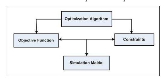
Figure 2 Linked Simulation-Optimization Methodology.
Gradient based optimization algorithms require derivatives of the objective and the constraint functions. In the LSO methodology, most of this information is not available. As a result, the optimization algorithm approximates the derivatives using conventional finite difference approximations. For n control variables, there are a total of n+1 functional evaluations of the objective function per iteration; this assumes a conventional forward difference approximation is used. The Jacobian of the constraints presents a more formidable problem. For m state variable constraints, there are (m x n) + 1 functional evaluations per iteration.
The principal advantage of the linked simulation-optimization methodology is its universality. In principal, highly nonlinear groundwater systems can be optimized for planning, design, or operational studies. The major disadvantage is computational. The finite difference approximations of the gradients and possibly the Hessian require extensive computational resources. In highly nonlinear problems there is also the problem of successfully identifying locally optimal solutions. Moreover, the state variable tradeoffs are not generated in the linked simulation-optimization approach.
4.2.1 LSO Application Sharp Interface Model
The LSO methodology was applied to the saltwater intrusion in the Jakarta, Indonesia regional aquifer system. A plan view of the 2730 km2 basin is shown in Figure 3. The aquifer systems are detailed in Figure 1.
Figure 3 The Jakarta Basin [1]
The groundwater basin is roughly coincident with the Quaternary sedimentary basin. A second formation, located on the slopes of the southern mountains, is continuous to the Jakarta basin and forms a regional aquifer composed of older Quaternary deposits south of Bogor. The third unit is located on the margins of the eastern and western mountains and comprises the impermeable basement formation of the region.
The Jakarta groundwater basin consists primarily of alluvial or deltaic sand and volcanic breccia separated by aquitards (semi-permeable aquifers). As shown in Figure 1, the uppermost aquifer in the system is unconfined, with an approximate thickness of 50 m. The aquifer overlays a series of deeper leaky aquifers at depths ranging from 50 to 250 m.
The development of the LSO solution of the optimal control model is predicated on a multi-aquifer sharp interface [5]. The calibration of the model is discussed in Samsuhadi [29].
The control model is similar to that presented in Eqs. (9)-(12). Both well injection (artificial recharge) and pumping bounds were incorporated in the model. In addition, water demands were maintained over each of the model's planning periods.
The objective used in the Jakarta optimization minimizes the sum of the squared saltwater volumes at the end of the planning horizon,
\[\min z = \sum_{\ell} \left[ \int \int \zeta_I^{\ell}(x, y) dx dy \right]^2 \tag{17}\] where the summation is over all layers, , of the groundwater system and is the location of the freshwater-saltwater interface. After considerable numerical experiments, this objective produced the most consistent and reliable optimization results, i.e. the sharpest objective gradients of the optimization model [29].
MINOS [30] was used for the solution of the optimization problem. Since the state variable of the model appears only in the objective function, the userdefined objective function was used to call the sharp interface model. The pumping and recharge decisions were passed from MINOS to the simulation model. The simulation model in turn generated the freshwater and saltwater heads, and the location of the freshwater and saltwater interface. The subroutines were called repeatedly in order to numerically approximate the gradient of the objective function.
Optimal pumping policies were developed for the Jakarta groundwater basin assuming steady-state hydraulics. The planning model considers a total of 104 different well locations for pumping and artificial recharge. The location of these well sites, developed in association with hydrogeologists from the Indonesian Ministry of Technology (BPPT), were located in the more permeable region of the groundwater basin.
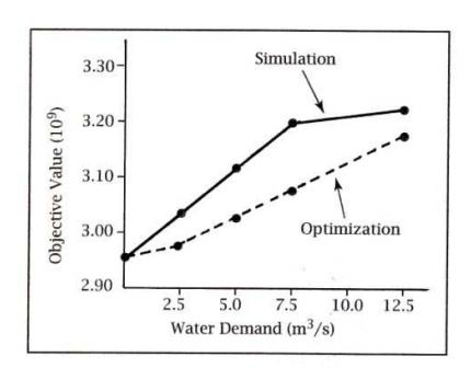
Figure 4 Saltwater and Demand Analysis.
An important set of optimization results is the tradeoff between the system objective, the total squared saltwater volume, and the water demand. Figure 4 summarizes the tradeoff as the water demand for the basin was varied from 0 to a maximum of \(12.5 \text{ m}^3/\text{sec}\).
The squared saltwater volume is a convex function of the water demand. For water demands up to \(3.6~\text{m}^3/\text{sec}\), the slope or shadow price of the curve (the change in the squared saltwater volume per unit change in the water demand) is approximately \(8.3~\text{x}~10^6~\text{m}^6/\text{m}^3/\text{sec}\). For demands exceeding \(3.6~\text{m}^3/\text{sec}\), the trade-off increases sharply to \(2.3~\text{x}~10^7~\text{m}^6/\text{m}^3/\text{sec}\). Increased water demands can be expected to dramatically increase the degradation (intrusion) occurring in the basin.
Also shown in Figure 4 is a comparison of the historical and optimized pumping schedules for various water demands (the simulated pumping schedules were determined from historical data). In all cases, the optimized pumping schedules significantly decrease the squared saltwater volumes. For example, with a water demand of 7.5 m³/sec, the simulated pumping pattern produces a total squared saltwater volume of approximately \(3.203 \times 10^9\) m⁶. The optimized pumping and recharge schedules decrease the objective to \(3.062 \times 10^9\) m⁶. The pumping and recharge pattern follows the same pattern as the historical demand schedule. Pumping is increased in layer 3 and decreased in layers 1 and 2. Artificial recharge also occurs in the aquifer system. The optimized pumping schedule generally increases the coastal head levels by shifting the groundwater pumping pattern and permitting artificial recharge.
4.2.2 LSO Application Density Dependent Saltwater Intrusion
A simple example of density-dependent transport optimization is the control of saltwater intrusion in a confined coastal aquifer. Figure 5 depicts the aquifer system. Recharge occurs along the left boundary of the system; a hydrostatic (saltwater) pressure distribution is maintained on the seawater boundary. Any fluid entering the system across this boundary is seawater, i.e. the concentration is [kg(dissolved solids/kg(seawater)]. The upper and lower boundaries of the system are confined. The initial saltwater distribution in the aquifer is zero. As shown in Figure 6, a series of pumping wells are located in the groundwater basin; the wells are screened in the upper portion of the aquifer. Table 1 summarizes the parameters of the model.
| Parameter | Value | Parameter | Value | |
|---|---|---|---|---|
| Porosity | 0.35 | Density ( ) | 700 [kg/m3 ] | |
| Seawater Density | 1025 [kg/m3 ] | Recharge | 0.066 [m3 /s] | |
| Long. Dispersivity ( ) | 0.0 | Trans. Dispersivity ( ) | 0.0 | |
| Permeability (k) | 1.020407.E-9 | Dm | 6.6.E-6 [m2 /s] | |
| [m2 ] | ||||
Table 1 SUTRA LSO Parameter.
The simulation model used in the analysis is SUTRA [28]. The initial data set is a test problem for the finite element model. The system, which is used for model verification of Henry's problem, consists of 231 nodes and 200 finite elements. The time step of the model is 1 minute; the total time simulation time is 100 minutes.
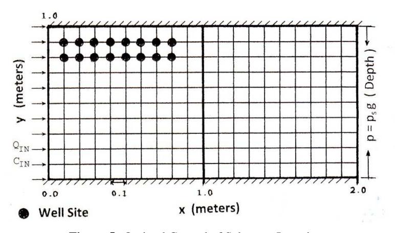
Figure 5 Optimal Control of Saltwater Intrusion.
The management of the coastal aquifer involves both the control of saltwater intrusion and the development of the aquifer as a source of water supply. Two optimization models are presented that address these issues. The first model minimizes the sum of the saltwater concentrations, , at the pumping wells, or
\[\min z = \sum_{i \in \pi} c_i \tag{18}\] where is an index set containing the coordinates of the wells. The optimization is constrained by the response equations (the SUTRA simulation
model that generates the concentration and pressure fields) and a water demand limitation
\[\sum_{i \in \pi} Q_i \ge D, \ Q_i \ge 0, \, \forall i \tag{19}\] where is the water demand for the basin.
The second model views the optimization somewhat differently. The objective is to maximize the sum of the total withdrawals from the system, or
\[\max z = \sum_{i \in \pi} Q_i \tag{20}\]
The constraints again include the response equations and explicit water quality constraints at each pumping well,
\[c_i \le c^*, \ \forall i \in \pi \tag{21}\] where is the allowable (standard) concentration. The extractions are also limited by the pump capacity, , and non-negativity,
\[0 \le Q_i \le Q_{i,\max}, \, \forall i \in \pi \tag{22}\]
The optimization models were solved using the LSO in conjunction with MINOS.
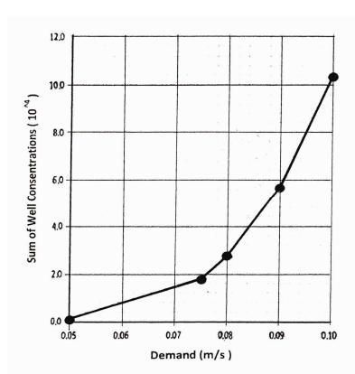
Figure 6 Sum of Well Concentration and Water Demand.
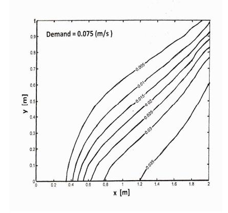
Figure 7 Isochlor Contour, Demand = 0.075 m/s.
The results of the first optimization model are summarized in Figures 6-7. Figure 6 depicts the sum of the well concentrations (mass fractions) versus the water demand. The tradeoff, the change in the well concentrations over the water demand [ ], varies from 0.00285 (demand = 0.05 [m/s]) to 0.047109 (demand = 0.09 [m/s]). The nonlinear variation in the tradeoff is typically of saltwater intrusion problems.
Figure 7 illustrates the steady-state salinity profile for a baseline demand of 0.075 [m/s].
The results of the 2nd optimization model are presented in Figures 8-9. Figure 8 is the tradeoff between the total extraction and the pumping upper bound, . The water quality is constrained to satisfy the standard, . In contrast to the first optimization, the tradeoff curve is linear for demands not exceeding 0.004 m/s.
The steady-state salinity profile for a well capacity of 0.003 [m/s] is illustrated in Figure 9.
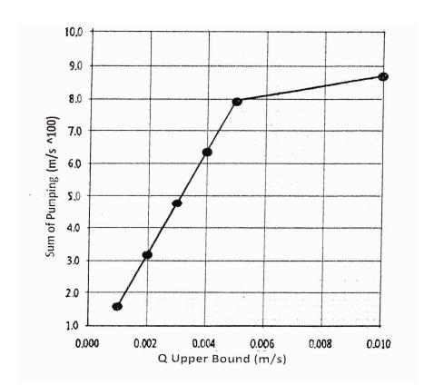
Figure 8 Total Pumping and Pumping Upper Bound.
Figure 9 Isochlor Contour, Concentration = 0.001, Q Upper Bound = 0.003 m/s.
The LSO methodology also facilities sensitivity analysis. The intrinsic permeability, boundary condition fluxes, and well locations can be easily varied within the optimization. The impacts and, importantly, tradeoffs can be directly assessed from the results of the optimization analysis. Again, this contrasts markedly with simulation where trial-and-error methods are used repeatedly to develop approximate solutions to the salinity control problem.
4.2.3 Other LSO Applications
A simulation-optimization methodology was used by Nishikawa [31] for the management of the water resources of Santa Barbara, California during drought conditions. MODFLOW was used to approximate the flow region; equivalent freshwater heads were used to represent the seawater boundaries.
Reichard [32] also presents a combined simulation-optimization model for the management of groundwater and surface water. A simulation model, developed by the California Department of Water Resources, is used to simulated groundwater flow in the Santa Clara–Calleguas basin. Saltwater intrusion is simulated using a particle tracking model. Particle velocities are determined from the transient water levels produced by the groundwater simulation model. The objectives addressed in the study were to minimize (1) supplemental water, (2) imported water, and (3) the change from existing groundwater conditions.
Johnson, et al. [33] presented a similar study for sea water intrusion management in Los Angeles County, California. Again, MODFLOW was used to simulate the aquifer system. Optimization was used to minimize barrier injection costs while maintaining adequate protection against seawater intrusion.
Nishikawa and Reichard [34] extended Reichard's early work to incorporate density-dependent flow and mass transport. The simulation-optimization methodology was used to control saltwater intrusion.
Bhattacharjya and Datta [35] used the linked simulation- optimization methodology to develop solution for an optimal management of saltwater intrusion in coastal aquifers. In simulation part, the governing equations were approximated using Artificial Neural Network (ANN) model and in the optimization part, the optimum solutions were found using Genetic Algorithm (GA) method.
Battacharjya, et al. [36] continued to explore the appropriateness of using ANN in solving the governing equation of saltwater intrusion problem. Similar approach was used by Dhar and Datta in LSO problem [37].
4.2.4 Box's Algorithm Application
Box's algorithm was applied to the Jakarta saltwater intrusion problem [38,39]. There were several reasons why the algorithm was selected over conventional constrained optimization methods. First, the nonconvexity of the optimal control problem means there are potentially a great many locally optimal solutions. Secondly, the overall response surface is relatively flat [1]. Thirdly, the MINOS solution often terminated with unusually large reduced gradients. Function precision and finite difference parameters had little or no impact on the optimization results.
In contrast, Box's algorithm was an efficient algorithm for the solution of the optimal control problem. Solutions were approximately 20% "better" than the MINOS solutions, given the same starting points for the algorithms.
| Water Demand | Response | Stress | Layer 1 | Layer 2 | Layer 3 | z* |
|---|---|---|---|---|---|---|
| m3/sec | \((m^3/s)\) | \((m^3/s)\) | \((m^3/s)\) | \((10^9)\) | ||
| 0.0 | 2.953 | |||||
| 3.6 | Hist | Pump | 0.86 | 0.80 | 1.94 | 3.087 |
| 3.6 | Hist | Rech | 0.00 | 0./00 | 0.00 | 3.087 |
| 3.6 | Opt | Pump | 0.44 | 1.15 | 7.97 | 2.977 |
| 3.6 | Opt | Rech | 1.84 | 0.86 | 2.36 | 2.977 |
| 7.5 | Hist | Pump | 1.78 | 1.67 | 4.05 | 3.204 |
| 7.5 | Hist | Rech | 0.0 | 0.00 | 0.00 | 3.204 |
| 7.5 | Opt | Pump | 1.33 | 1.62 | 10.33 | 3.062 |
| 7.5 | Opt | Rech | 1.20 | 0.88 | 3.75 | 3.062 |
| 12.5 | Hist | Pump | 2.97 | 2.78 | 0.74 | 3.255 |
| 12.5 | Hist | Rech | 0.00 | 0.00 | 0.00 | 3.255 |
| 12.5 | Opt | Pump | 2.36 | 1.95 | 8.07 | 3.178 |
| 12.5 | Opt | Rech | 0.00 | 0.00 | 0.02 | 3.178 |
Table 2 Optimization Results Jakarta Groundwater Basin.
The algorithm was used to assess the optimality of the existing pumping pattern in the basin. Table 2 summarizes the historical and optimized pumping schedules for each aquifer system for three differing demand schedules. For example, with a water demand of 12.5 m<sup>3</sup>/s, the majority of the historical pumping schedule occurs in layer 3 of the aquifer system. Layers 1 and 2 contribute approximately the same total groundwater withdrawal, and there is no artificial recharge occurring in the basin. The total squared saltwater volume is approximately 3.26 x 10<sup>9</sup> m<sup>6</sup>. The optimization results decrease the total squared saltwater volume by approximately 6% over the historical value. Pumping increases in layer 3; layers 1 and 2 both show a decrease in the total volume of pumping. In contrast to the simulation results that represent the historical pumping pattern, the optimization introduces artificial recharge in layer 3 of the system. The magnitude of artificial recharge is 0.02 m<sup>3</sup>/sec.
In their recent work, Curtis and Willis [40] used LSO approach by combining Box's algorithm and HST3D in finding the optimal solution.
5 Conclusion
The objective of this paper was to present a summary of models for the optimal control of saltwater intrusion. The most general formulation of the water quality management problem is an optimal control model. The Imbedding approach, the linked simulation-optimization methodology, and Box's algorithm have been used to generate locally optimal planning alternatives for both density dependent and sharp interface models. The optimization approach, despite requiring significant computation resources, is superior to conventional
simulation methods. Optimization produces not only locally optimal planning, design, and operational policies, but also the tradeoffs associated with environmental and hydraulic objectives.
Acknowledgements
The authors wish to express their thanks to the Ministry of National Education of Indonesia (PAR-2011 DIKTI).