
1 Introduction
In geophysics, the gravity modeling method has been used for a wide range of applications, such as tectonic studies [1,2], earth resources exploration [3,4] and also in engineering and environmental investigations [5]. Gravity anomalies are generated by mass variations in subsurface rock formations. The aim of the gravity modeling is to estimate the densities and shapes (i.e. geometry, including depth) of the causative bodies. An inversion technique is usually employed to obtain a plausible subsurface model whose theoretical response (or calculated data) fits the observed data. Therefore, the inversion of gravity data constitutes an important step in the quantitative interpretation of gravity anomalies [6,7].
In two-dimensional (2D) modeling, a causative body with invariant crosssection along an assumed strike is sought with respect to the gravity data on a profile crossing perpendicularly to that strike. One of the possible approaches is to divide the subsurface into a large number of rectangular blocks of fixed size but of unknown density (see Figure 1). In such case, the density of each block is to be determined and the inversion problem is linear, i.e. the data or gravity anomalies are linearly related to the model parameters or densities [8,9]. A major difficulty with the inversion of gravity data (and other potential field data, such as magnetic field data) is the inherent non-uniqueness of inverse models. If a model is found to fit the data, there may be many other models that fit the data to the same degree [8-10].
This paper describes an alternative implementation of the constrained 2D gravity inversion that minimizes the moment of inertia of the causative bodies with respect to one or several axes passing through them. The approach used was proposed by Guillen and Menichetti [11] and by Barbosa and Silva [12,13] with a more generalized formulation. Their inverse model is determined by the estimate of the central depth and dip of the anomalous sources. We limit our approach by using explicit axis positions as a constraint in the inversion algorithm. Such constraint is a specific and rather restrictive form of prior information. However, the attempt to collapse the anomalous density into a single body (or multiple bodies with their respective axes) is more suited for recovering localized geological structures, for example in mineral exploration (i.e. dikes, sills, etc). This choice of preference will be exemplified by inversion of synthetic and field data.
2 Unconstrained 2D Gravity Inversion
The subsurface in which the anomalous sources are searched is divided into elementary rectangular prisms on the x- and z-axis (of infinite horizontal extent in the y-axis, i.e. 2D case). The elementary density contrasts are constant inside each prism and can vary individually. With the matrix notation, the vector of gravity anomaly d = [di] ; i = 1, 2, …, N with N is the number of data, is given by
\[\mathbf{d} = \mathbf{G} \cdot \mathbf{m} \,, \tag{1}\] where G = [gij] ; i = 1, 2, …, N ; j = 1, 2, …, M is the kernel matrix with gij is the contribution of j-th prism to the gravity value on i-th observation point. The vector for model parameters that represents the density contrast of the prism is m = [mj] ; j = 1, 2, …, M with M is the number of model parameters. The number of model parameters is factored as the number of prisms in the direction of the x- and z-axis (Figure 1).
Eq. (1) constitutes the 2D gravity forward modeling, i.e. to calculate the predicted gravity anomalies (or theoretical data d) for a known subsurface density contrast (or model m). The gravity response of an elementary prism gij is obtained from the well-known Talwani's algorithm, i.e. calculation of the gravitational attraction of an arbitrary 2D anomalous body with a polygonal
cross-section [10]. In this case, the polygon has four perpendicular sides that coincide with the model grids.
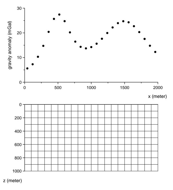
Figure 1 Illustration of the gravity anomaly data along a profile and associated 2D section with common x-axis. The subsurface domain on the x- and z-axis is discretized into grids representing 2D prisms.
Since the gravity observation points are located only at the earth's surface along a profile crossing the anomalous body, the number of model parameters is certainly larger than the number of data. For such under-determined problems, the standard minimum-norm solution of the inverse problem is expressed by [8,9]
\[\mathbf{m} = \mathbf{G}^T \left[ \mathbf{G} \, \mathbf{G}^T + \lambda \, \mathbf{I} \right]^{-1} \, \mathbf{d} \,, \tag{2}\] where \(\lambda\) is the damping factor, I is a unitary matrix and the super-script T denotes matrix transposition. The damping factor is used to avoid over-fitting, i.e. unnecessary model solutions that reproduce noise contained in the data. The choice of the damping factor is usually determined by trial and error. However, to minimize the ad hoc manner in the choice of the damping factor, Mendonca and Silva [14,15] used a normalization matrix D such that \(\lambda\) can be chosen in the interval [0, 1]. The N by N diagonal normalization matrix D is given by
\[D_{ii} = \left(\sum_{j=1}^{M} G_{ij}^{2}\right)^{-1/2},\tag{3}\] and the Eq. (2) becomes
\[\hat{\mathbf{m}} = \mathbf{G}^T \mathbf{D} \left[ \mathbf{D} \mathbf{G} \mathbf{G}^T \mathbf{D} + \lambda \mathbf{I} \right]^{-1} \mathbf{D} \mathbf{d}.\] (4)
In order to stabilize the inversion, the singular value decomposition (SVD) technique [16] is usually employed to invert the matrix in Eq. (2) or its modified or normalized version as shown in Eq. (4). In the application of the SVD technique, singular values less than a threshold value are considered negligible and set to zero such that they are discarded from the solution calculation. In the cases described in this paper, singular values less than \(10^{-6}\) times the maximum singular value are neglected, which resulted in good solutions. However, Eqs. (2) and (4) represent the unconstrained 2D gravity inversion, where the inverse model tends to concentrate near the earth's surface due to the ambiguity or non-uniqueness problem. This mathematical solution provides little information about the true structure. However, such situation can still be exploited in the context of an equivalent source for interpolation [14,15] and also for potential field data transformation [17].
3 Constrained 2D Gravity Inversion
Several authors have introduced prior information into the inversion in order to restrict the number of solutions and to reflect the actual geology of the area. In such approach, the inversion algorithm produces a single model by minimizing an objective function of the model subject to fitting the data. For example, Li and Oldenburg [18] used an objective function that includes terms penalizing discrepancies from a reference model and also roughness in three different spatial directions (x, y, z). It also incorporates a depth weighting function designed to distribute the density with depth. Their inversion technique has the ability to construct relatively complex (3D) geologic bodies. However, the inverted models tend to exhibit remarkably smooth models so that the determination of rock boundaries is a difficult interpretation task.
We consider a class of models most likely encountered in real geophysical exploration problems for mineral resources employing the gravity modeling method. We search for anomalous sources collapsed into bodies with their axis defined as "a priori" information. This approach is a simplified implementation of the more generalized method proposed by Guillen and Menichetti [11] and also by Silva and Barbosa [12] that incorporates only the center of gravity and orientation (dip) of the axes as constraints. Instead of automatically finding the extent of the anomaly along the predefined axis orientation (i.e. the axis' length), we use the explicit position of the axes by defining their extreme points as constraints.
For inversion with a known position of axes, the model parameter estimate is updated iteratively; at the k-th iteration we have
\[\mathbf{m}^{k+1} = \mathbf{m}^k + \Delta \mathbf{m}^k, \tag{5}\]
\[\Delta \mathbf{m}^{k} = \mathbf{W}_{k}^{-1} \mathbf{G}^{T} [\mathbf{G} \mathbf{W}_{k}^{-1} \mathbf{G}^{T} + \lambda \mathbf{I}]^{-1} (\mathbf{d} - \mathbf{G} \mathbf{m}^{k}),\] (6)
\(\mathbf{W}_k\) is a diagonal weighting matrix and its non-zero elements are given by
\[w_{jj} = \frac{R_j^2}{m_j^k + \varepsilon},\tag{7}\]
\[R_j = \min_{1 < i < L} (r_{ij}), \qquad (8)\] where \(r_{ij}\) is the distance between the center of the j-th elementary prism and the i-th axis, and \(\varepsilon\) is a small positive number in the order of \(10^{-7}\) to avoid a division-by-zero error in Eq. (7) for zero density contrast in the model parameter. The form of Eq. (6) is similar to that of Eq. (2) for general minimum-norm solutions of the linear inverse problem. Eq. (6) gives the constrained model perturbation that can be used to update the model parameters (i.e. density or density contrast) iteratively. In Silva and Barbosa [12], a lengthy formulation was necessary to evaluate the weighting matrix elements since the constraints were the center gravity and the dip or orientation of the axes.
The algorithm of the proposed method is as follows:
- Calculation of the standard minimum-norm solution. The calculation of the minimum-norm solution using Eq. (4) always results in an acceptable fit of the data. However, the solution does not support the real subsurface geology nor the predefined constraints, i.e. the concentration of mass about the specified axes.
- 2. Calculation of weighting matrix W. The components of the matrix W evaluated using Eqs. (7) and (8) will control the modulus of the perturbation \(\Delta \mathbf{m}\) at each iteration. The prisms close to any axis that have large density contrast estimates (in the modulus)
are assigned small weights, so that the corresponding corrections will be large, and vice versa.
3. Application of inequality constraints on density.
To produce a physically meaningful solution, the density contrast of each prism must satisfy
\[m_{\min} \le m_j \le m_{\max}\] (9)
If at an iteration mj exceeds one of its bounds, then it will be fixed at the violated bound. Instead of being calculated by Eqs. (7) and (8), the corresponding weight wjj will be assigned a very large value. The large value for wjj will force the prism density contrast to be "frozen" at the violated boundary, at least temporarily during the first few iterations. This way, the response of the modified parameter estimates will not fit the observations, which will in turn trigger the necessity for further parameter perturbation as a function of the misfit.
4. Calculation of model perturbation and model updating.
The calculation of Eqs. (6) and (5) will result in the density contrast perturbation and an updated density contrast model respectively. The iterations continue with the re-evaluation of the weighting matrix W in step (2) and so forth. The model will be biased towards a concentrated density contrast estimate close to the axes, which will likely outline the causative bodies.
4 Inversion of Synthetic Data
To illustrate the utility of the proposed method, the inversion algorithm was tested on a set of synthetic data. The gravity field of the 2D prisms having a simple geometry and also an irregular form is most likely encountered in mineral exploration (dikes and sills); it was computed by Talwani's method [10]. The density contrast of the anomalous body is 1.0 gr/cm3 . The synthetic data were contaminated by random noise with a Gaussian distribution having zero mean and a standard deviation of 1.0 milliGal. We worked with gravity anomalies and density contrasts instead of gravity fields and densities. Since the only unknown parameters were the contrasts of density, the anomalous bodies were represented by the prisms with non-zero contrast. The modeling domain was decomposed into 40 by 20 blocks with a dimension of 50 meters in both xand z-direction.
In the inversions, we used a subsurface discretization similar with the one used in generating the synthetic data in order to simplify the problem. The density contrast was bounded between 0.0 and 1.0 gr/cm3 . Figure 2 shows the results from the unconstrained inversions of the synthetic data corresponding to the bodies with a simple geometry (horizontal and vertical blocks). Despite the good fit between the calculated data and the observed data, the recovered causative bodies do not reflect the real geometry of the synthetic models (shown as outline in the model cross-section). The inverted models tend to concentrate near the surface with a much lower density contrast than prescribed in the synthetic models. Note also the negative density contrast (white colored blocks at the surface and near the edges) that compensates the non-zero density contrast of blocks that are too close to the surface.
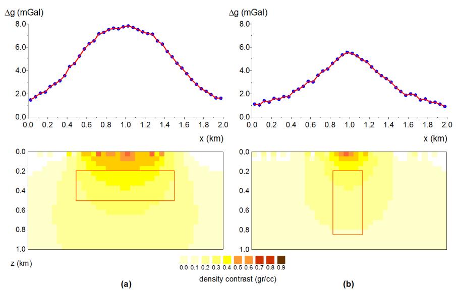
Figure 2 Unconstrained inversion results of synthetic data associated with horizontal block (a) and vertical block (b) synthetic models. The corresponding fits between synthetic data (dots) and calculated data (line) are shown in the top panel.
The constrained inversion of the same synthetic data, by giving the axis position of the presumable anomalous mass, resulted in a much better geometry of the inverted models (Figure 3). In inverting each synthetic data set, the true axis at the center of the synthetic model was given. The level of data fit for both the unconstrained and constrained inversions are almost identical. However, the calculated model response from the constrained inversion appears to be smoother, due to the fact that the inverse model is less irregular than the model obtained from the unconstrained inversion. For the same degree of damping, the inversion without appropriate constraint tends to overfit the data including the noise present in the data.
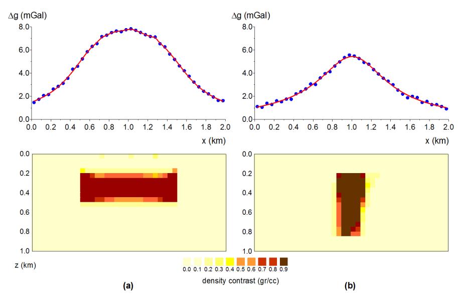
Figure 3 The constrained inversion results of synthetic data associated with horizontal block (a) and vertical block (b) models. The corresponding fits between synthetic data (dots) and calculated data (line) are shown in the top panel.
We also inverted synthetic data associated with anomalous bodies having a more complex geometry in order to investigate the validity of the inversion algorithm and the critical choice in setting the axis position for the constraint. The inversion without constraint was performed but we do not present the results in this paper since the inverse model exhibited similar characteristics as in Figure 2, i.e. no significant physical or geological structures were obtained. Figure 4 shows the inversion results for synthetic data corresponding to combinations of dikes and sills with orthogonal and inclined crossing axes. This figure also depicts good agreement between recovered and synthetic models both in terms of geometry and density contrast. As with the previous inversions of synthetic data, the true axes at the center of the synthetic models (both orthogonal and non-orthogonal) were given as constraints (shown as arrows in Figure 4) in order to simplify the problem.
Inversions using an incorrect position of the axes were also performed (not presented in this paper) to test the sensitivity of the method under such
condition. They resulted in models that are geologically unrealistic, although the data misfit may be acceptable. Such kind of results can be used as an indicator that the constraints are inappropriate and further adjustment of the axes' positions is still needed.
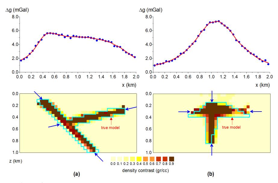
Figure 4 The constrained inversion results of synthetic data associated with models having two crossed axes (a) and (b), with their corresponding fits between synthetic data (dots) and calculated data (line). The arrows are the axes given as constraints.
5 Inversion of Field Data
The proposed method was applied to invert field gravity data from a private concession for artisanal gold mining operated by a local community in the southern part of Sukabumi regency, West Java province, Indonesia. The objective of the survey was to delineate the mineralized zone associated with an intrusive dike that is generally denser than its surrounding environment. As a by-product of the intrusion, the mineralization that occurs in the quartz veins may contain gold as ore, although usually in very small quantities. The survey area, measuring only 900 by 600 meters in East-West and North-South directions respectively, was covered by gravity stations in grids of 50 by 50 meters. For such a small and localized area, we only performed relative Bouguer gravity measurement, i.e. no tie to the regional base-station. A simple constant regional anomaly was substracted from the Bouguer anomaly. Figure 5
shows the residual anomaly map in a simple local x-y Cartesian coordinate system.
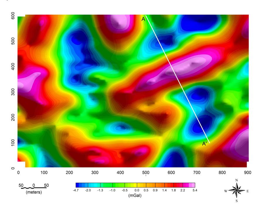
Figure 5 The residual gravity anomaly from the survey area. The modeled data were from the profile shown by white line crossing the main positive anomaly.
The residual gravity exhibits a dominant positive anomaly in South-West – North-East direction surrounded by lower and negative anomalies. We inverted the data from a profile A-A' in nearly North-West – South-East direction crossing the main positive anomaly perpendicularly. The subsurface domain was divided into 40 by 20 blocks with a dimension of 25 meters in both x- and z-direction. The results of the unconstrained and constrained inversions are presented in Figure 6. The unconstrained inversion resulted in a diffuse anomalous source concentrated near the surface with a good fit between the observed data and the calculated data. After several attemps, the best result for the constrained inversion in terms of data fit and model continuity was obtained by using a vertical axis as shown by the blue arrow in Figure 6(b). The difficulty in achieving a good data fit may be caused by the limited density contrast for the anomalous body. The boundary of the anomaly is well resolved, although the anomalous body is still concentrated near the surface. The fact that the anomalous body does not have an intrusive character, i.e. is not deeply
rooted, is intriguing. For such a local anomaly, it is possible that we covered the whole intrusive system only partially. The main instrusive body may be located elsewhere, further to the North-East of the survey area.
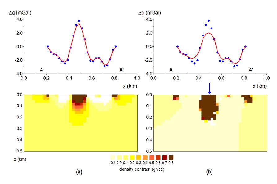
Figure 6 The unconstrained (a) and constrained (b) inversion results of the field data (dots) with their corresponding calculated model response (line). The arrow in Figure 6(b) is the axis given as constraint.
6 Discussion and Conclusion
An inversion algorithm to recover 2D contrast density distribution from gravity data was presented. The algorithm incorporates constraints about the directions of the mass concentration in order to obtain a mathematically stable and physically and geologically meaningful solution. In order to simplify the problem, the applied constraint was given explicitly as the coordinate points of the axes. The versatility of such constraints in the algorithm was exemplified by inversion of synthetic data. The inverse models successfully recovered the synthetic models within an acceptable resolution. The inversion of the field gravity data also resulted in a satisfactory subsurface model.
The need for rather specific "a priori" information, such as the axis of the anomalous body, seems restrictive and may prohibit the application of the algorithm in solving real geological exploration problems. The experiment with false constraints or weak "a priori" information has shown that the applicability of the proposed method is not restricted to areas with a relatively well-known geology. Nevertheless, in an exploration program it is rare that little or nothing is known about the local geology. This suggests that relatively reliable "a priori" information is usually available to perform inversion modeling properly using the method proposed in this paper.
From a computational point of view, the numerical implementation of the algorithm can be as efficient as other techniques employing constraints on model smoothness, depth weighting, etc. [18]. The minimum-norm (i.e. underdetermined) type of the inverse problem resolution leads to a matrix inversion whose size is determined by the number of observations rather than by the number of model parameters (prisms or grids). The current computational resources are appropriate to handle such inversion modeling routinely, even with a large number of grids. The extension of the algorithm to solve more complex 3D structures is currently underway based on existing 3D gravity and magnetic modeling algorithms [19]. The development of the algorithm for 3D inversion of magnetic data is crucial since magnetic data are used more frequently in mineral exploration.