1 Introduction

Quantum computing is one of the most promising developments in computer science. It involves the application of the quantum mechanics paradigm to computation and it is believed to have the power to solve problems that are unsolvable in classical computing. In computer science, one class of these problems is known as NP-complete problems. There are many problems which belong to the class of NP-complete problems, e.g. k -SAT, travelling salesman problems, factoring, etc. A classical computer will have difficulties solving these problems because the computation is performed serially. Quantum mechanics solves problems by the superposition principle, which allows the calculation to be done in parallel naturally. This feature makes quantum computing more powerful [1].

One way to perform quantum computing is to use the quantum adiabatic theorem. This approach, known as adiabatic quantum computing (AQC), was proposed by Farhi [2] to solve 3-SAT problems. Some progress in AQC has been made to solve NP-complete problems, such as finding low-energy conformations of lattice protein models [3], search engine ranking [4], random SAT [5], quantum search [6-9], and the famous travelling salesman problems [10]. If in conventional quantum computing [2], one uses a sequence of quantum gates, in AQC one uses the adiabatic evolution of an initial Hamiltonian to a final Hamiltonian that encodes the solution of the problem.

Some researchers [11] have also realized Hamiltonians to implement universal adiabatic quantum computers. In addition, other researchers [12,13] also have shown that AQC is equivalent to standard quantum computing. Besides the effort in developing time-dependent Hamiltonians encoding the solution of the problems, there is a growing interest in analysing and improving the computation time in adiabatic computation. There are some ways to speed up computation time in AQC, such as adding an extra piece of Hamiltonian [14-16], modifying the Hamiltonian [17], or choosing suitable interpolation functions [18,19].

From the researches mentioned above, we can conclude that there are two major research problems in AQC: firstly, dealing with the problem of how to develop a Hamiltonian that can encode the solution of a given problem, and secondly, finding a way to speed up computation, e.g. by choosing suitable interpolation functions. As mentioned before, the objective of choosing a suitable interpolation function is to optimize or minimize the computation time. This interpolation function is called 'time functional' because it depends on the scaled time [19,20]. The time functional depends on the energy gap between the two lowest energy levels as well as on the rate of change of the time-dependent

Hamiltonian \[\left|\left\langle \Phi_{m}(s)\right| \frac{d\mathcal{H}(s)}{ds} \middle| \Phi_{n}(s) \right\rangle\]. In [2] this second part is assumed to be bounded \[0 < \left| \left\langle \Phi_m(s) \right| \frac{d\mathcal{H}(s)}{ds} \middle| \Phi_n(s) \right\rangle \right| \le 1\]. In [20] this latter part is expressed in a

Hilbert-Schmidt (or Frobenius) norm, and it is known that it is very hard to evaluate and compute this expression for a general Hamiltonian, even numerically [19].

In general, one can formulate the problem as a variational optimization problem that can be solved using the standard Euler-Lagrange equation. In this work we have computed the evolution paths for the original ACQ problem as well as for the problem with additional Hamiltonian. Specifically, we have implemented this for the case of a Hadamard gate.

This paper is organized as follows: in Section 2 we review the basic idea of AQC and in Section 3 reformulate the time functional in its original form. In Section 4 we calculate the paths for various problems as mentioned above. The conclusion is given in Section 5.

2 Adiabatic Theorem for Quantum Systems

The dynamics of a quantum system are described by the time-dependent Schrödinger equation

\[\mathcal{H}(t)|\Psi(t)\rangle = i\hbar \frac{d}{dt}|\Psi(t)\rangle. \tag{1}\]

The time-dependent Hamiltonian \(\mathcal{H}(t)\) is a normal operator [21] that is acting on a non-degenerate ground state [20] \(|\Phi_n(t)\rangle\) according to

\[\mathcal{H}(t)|\Phi_n(t)\rangle = E_n(t)|\Phi_n(t)\rangle. \tag{2}\]

According to the adiabatic theorem, if the Hamiltonian varies slowly in the range [t,T] and there is a fairly large energy gap between the ground state and the first excitation, then the system is guaranteed to stay in the ground state at the end of the evolution. If we assume the eigenstates are orthonormal, then the fidelity is given as follows [21]

\[F(t) = \left| \left\langle \Phi_n(t) | \Phi(T) \right\rangle \right|^2 = 1 - \sum_{l \neq n} \left| \left\langle \Phi_l(t) | \Phi(T) \right\rangle \right|^2 = 1 - \varepsilon^2, \tag{3}\] where \(\varepsilon \ll 1\).

Now, suppose that the solution to the time-dependent Schrödinger equation is

\[\left|\Psi(t)\right\rangle = \sum_{n} c_{n}(t) e^{-i\frac{1}{h} \int_{0}^{t} E_{n}(\tau') d\tau'} \left|\Phi_{n}(t)\right\rangle. \tag{4}\]

If we substitute this expression into Eq. (1) and then multiply it by \(\langle \Phi_{m}(t) |\), we get

\[\dot{c}_n = \sum_n c_n(t) \langle \Phi_m(t) | \dot{\Phi}_n(t) \rangle e^{i \int_0^t \omega_{mn}(\tau') d\tau'}, \tag{5}\] where \(\omega_{\rm mn}=\frac{E_{\rm m}(\tau)-E_{\rm n}(\tau)}{\hbar}\). Meanwhile, after differentiating Eq. (2) and multiplying it by \(\langle\Phi_{\rm m}(t)|\) we get

\[\left\langle \Phi_{m}\left(t\right) \middle| \dot{\Phi}_{n}\left(t\right) \right\rangle = \frac{\left\langle \Phi_{m}\left(t\right) \middle| \dot{\mathcal{H}}\left(t\right) \middle| \Phi_{n}\left(t\right) \right\rangle}{E_{m}\left(t\right) - E_{n}\left(t\right)}.\] (6)

Substitute this equation into Eq. (5) and then integrate with initial condition \(c_{0n}(0) = \delta_{0n}\) to yield

\[c_n = \delta_{0n} + \sum_{m \neq n0} {}^t c_m(t) e^{i \int_0^t \omega_{mn}(\tau') d\tau'} \omega_{mn}(\tau) K_{mn}(\tau) d\tau\] \[(7)\] with \(K_{mn}(\tau) = \hbar \frac{\langle \Phi_m(\tau) | \dot{\mathcal{H}} | \Phi_n(\tau) \rangle}{(E_m(\tau) - E_n(\tau))^2}\). The first order approximation of \(c_n\) gives

\[c_n^{(1)} = \int_0^t e^{i \int_0^t \omega_{0n}(\tau') d\tau'} \omega_{0n}(\tau) K_{0n}(\tau) d\tau.\] (8)

After integrating by parts and then substituting it into Eq.(4) we have

\[|\Psi(t)\rangle = \sum_{n} c_{n}(t)e^{i\theta_{n}} |\Phi_{n}(t)\rangle\] \[= -i\hbar \frac{\langle \Phi_{m}(t)|\dot{\mathcal{H}}(t)|\Phi_{n}(t)\rangle}{(E_{m}(t) - E_{n}(t))^{2}} e^{i\int_{0}^{t} \omega_{0n}(\tau')d\tau'} |\Phi_{n}(t)\rangle. \tag{9}\]

Our calculation leads us to the following simple conclusion: If we prepare a quantum system on a ground state (given by Eq.(4)) and we evolve it according to Schrödinger Eq. (1) and the eigen Eq. (2), the system will remain in its ground state (given by Eq. (9)).

3 Evolution Path in AQC

In the previous section we have discussed the adiabatic theorem of a quantum system given by Eq. (9). The transition probability is given by Eq. (9)

\[P(t) = \left| -i\hbar \frac{\left\langle \Phi_m(t) \middle| \dot{\mathcal{H}}(t) \middle| \Phi_n(t) \right\rangle}{\left( E_m(t) - E_n(t) \right)^2} e^{i \int_0^t \omega_{0n}(\tau') d\tau'} \right|^2. \tag{10}\]

In order for the system to remain in the ground state at the end of the evolution, \(P(t) \ll 1\). This is guaranteed by the value of \(\hbar\), so we have

\[1 \gg \frac{\left\langle \Phi_m(t) \middle| \dot{\mathcal{H}}(t) \middle| \Phi_n(t) \right\rangle}{\left( E_m(t) - E_n(t) \right)^2}. \tag{11}\]

Define the evolution time scale as \(s(t) \equiv t/T\), then Eq. (11) gives the time functional

\[T = \int_{0}^{1} \frac{\left\langle \Phi_{m}(s) \middle| \frac{d\mathcal{H}(s)}{ds} \middle| \Phi_{n}(s) \right\rangle}{\left( E_{m}(s) - E_{n}(s) \right)^{2}} ds. \tag{12}\]

The time functional defined in Eq. (12) should be minimized to get the expected speed-up in the AQC paradigm, which can be done by solving the Euler-Lagrange equation

\[\frac{d}{ds} \left( \frac{\partial L}{\partial \dot{x}} \right) = \frac{\partial L}{\partial x} \tag{13}\] with the 'Lagrangian' defined as

\[L = \frac{\left\langle \Phi_m(s) \middle| \frac{d\mathcal{H}(s)}{ds} \middle| \Phi_n(s) \right\rangle}{\left( E_m(s) - E_n(s) \right)^2}.\] (14)

It is very hard to solve the Euler-Lagrange equation analytically [19]. One attempt in [20] is to write the expectation value of \(\langle \Phi_m(s) | \frac{d\mathcal{H}(s)}{ds} | \Phi_n(s) \rangle\) as a norm form. If we use the norm form for our case, we cannot find the function that minimizes the time functional because the Euler-Lagrange equation always vanishes, i.e. the solution is an arbitrary function. In the next section we will modify the evolution path by adding an extra Hamiltonian.

Now, we will compute the AQC interpolation function proposed by [2]. The linear interpolation of a time-dependent Hamiltonian proposed by [2]

\[\mathcal{H}(s) = (1-s)\mathcal{H}_s + s\mathcal{H}_s, \tag{15}\]

can be generalized as follows

\[\mathcal{H}(f(s),g(s)) = f(s)\mathcal{H}_i + g(s)\mathcal{H}_f, \tag{16}\] where f(0) = g(1) = 1 and f(1) = g(0) = 0. To simplify the writing later, the s dependence of the interpolation function is not written explicitly.

As is well known, the initial and final Hamiltonians can be constructed from the orthonormal basis vectors. For example, using two orthonormal states, \(|\xi\rangle\) and \(|\varphi\rangle\), one can construct

\[\mathcal{H}_{i} \equiv -|\xi\rangle\langle\xi| + |\phi\rangle\langle\phi|,\tag{17}\]

\[\mathcal{H}_{f} \equiv |\xi\rangle\langle\phi| + |\phi\rangle\langle\xi|. \tag{18}\]

For simplicity, in a one qubit system we have

\[\left| \xi \right\rangle \equiv \left| 0 \right\rangle = \begin{pmatrix} 1 \\ 0 \end{pmatrix} \tag{19}\]

\[\left|\boldsymbol{\varphi}\right\rangle \equiv \left|1\right\rangle = \begin{pmatrix} 0\\1 \end{pmatrix}. \tag{20}\]

On this basis, the initial and final Hamiltonians are written as

\[\mathcal{H}_i = \begin{pmatrix} -1 & 0 \\ 0 & 1 \end{pmatrix},\tag{21}\]

\[\mathcal{H}_f = \begin{pmatrix} 0 & 1 \\ 1 & 0 \end{pmatrix}, \tag{22}\] and the eigenvalues and eigenvectors of the time-dependent Hamiltonian (16) are

\[\lambda = \pm \sqrt{f^2 + g^2} \tag{23}\]

\[\left|\Phi_{m,n}(s)\right\rangle = \left(\frac{\pm \left|\lambda\right| - f}{g}\right).\] (24)

Therefore the 'Lagrangian' is given by

\[L = -\frac{f\dot{g}}{2|\lambda|^2 g} - \frac{f^2 \dot{f}}{4|\lambda|^2 g^2} + \frac{\dot{f}}{4|\lambda|^2} + \frac{\dot{f}}{4g^2},\] (25)

from which, using Eq. (13), we get the Euler-Lagrange equations for the interpolation functions f and g, respectively,

\[f^2 \dot{g} + g^2 \dot{g} = 0, (26)\]

\[f^2\dot{f} + g^2\dot{f} = 0. (27)\]

Solving these equations subject to the boundary conditions yields

\[f = 1 - g. (28)\]

The scenario of adding an extra Hamiltonian to modify the evolution path to obtain a speed-up in AQC has been discussed in [14-16]. We will use this idea to modify the path and choose the extra Hamiltonian to be

\[\mathcal{H}_{e} \equiv k \mathcal{H}_{f} \tag{29}\] where k is a number taken to be integer for convenience. The time-dependent Hamiltonian now becomes

\[\mathcal{H}(s) = f\mathcal{H}_i + g\mathcal{H}_f + h\mathcal{H}_e, \tag{30}\] in which the interpolation function h(s) that controls the extra Hamiltonian satisfies h(0) = h(1) = 0. The eigenvalues and eigenvectors of this Hamiltonian are

\[\lambda = \pm \sqrt{f^2 + g^2 + k^2 h^2 + 2kgh} \tag{31}\]

\[\left|\Phi_{m,n}(s)\right\rangle = \left(\frac{1}{\pm |\lambda| - f}, \atop kh + g, \right), \tag{32}\] and the 'Lagrangian' is given by

\[L = -\frac{f(k\dot{h} + \dot{g})}{2|\lambda|^{2}(kh + g)} - \frac{f^{2}\dot{f}}{4|\lambda|^{2}(kh + g)^{2}} + \frac{\dot{f}}{4|\lambda|^{2}} + \frac{\dot{f}}{4(kh + g)^{2}}.\] (33)

The Euler-Lagrange equations are (see Appendix for more details)

\[[f^{2} + (kh + g)^{2}](kh + g)^{2}(k\dot{h} + \dot{g}) = 0,\] (34)

\[[f^{2} + (kh + g)^{2}](kh + g)^{2}\dot{f} = 0.\] (35)

All solutions to the above equations fail the boundary conditions, which means that the performance does not depend on the choice of function h(s). It will, however, depend on the choice of the extra Hamiltonian.

4 Implementation of Hadamard Gate

The Hadamard gate is defined as [1, 22]

\[\mathcal{H} = \frac{1}{\sqrt{2}} \begin{pmatrix} 1 & 1\\ 1 & -1 \end{pmatrix},\tag{36}\] which transforms \(\mathcal{H}_{t} = -\sigma_{z}\) to \(\mathcal{H}_{f} = -\sigma_{x}\) [22], i.e.

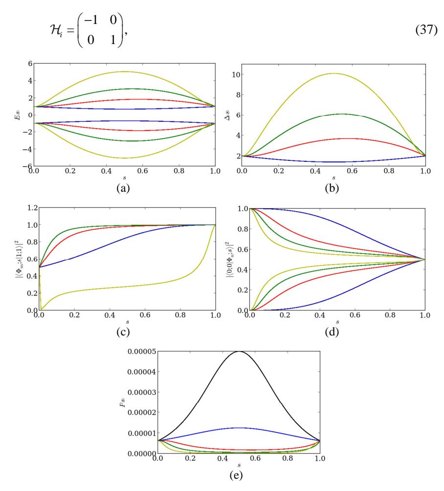
Figure 1 Performing AQC to implement a Hadamard gate with original Hamiltonian (black line) and extra Hamiltonian. Blue, red, and green lines for k=5, k=10 and k=20 respectively. The yellow line is for the extra Hamiltonian of Pauli operator \(\sigma_y\) with k=20.

\[\mathcal{H}_f = \begin{pmatrix} 0 & -1 \\ -1 & 0 \end{pmatrix}. \tag{38}\]

It can be easily checked that these initial and final Hamiltonians are the inverses of the previous initial and final Hamiltonians, so we would have the same results as before. The result of AQC implementation of a Hadamard gate with g(s) = s is given in Figure 1.

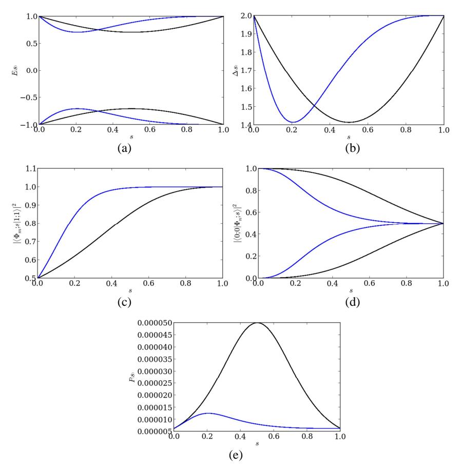
Figure 2 AQC implementation of a Hadamard gate with linear (black line) and cubic \(g(s) = s^3 - 3s^2 + 3s\) (blue line) interpolation functions.

In Figure 1 the black line is for h(s) = 0, while the blue, red, and green lines are for evolution paths with an extra Hamiltonian. The yellow line is the result for taking Pauli operator^{σ y} as the extra Hamiltonian. The two lowest energy levels and their gap are given in Figure 1(a) and (b). The fidelity of the evolving state with respect to the ground state is given in Figure 1(c), which becomes unity at the end of the evolution as it should. The mixture and transition probabilities of the ground state and the first exited states are given in Figure 1(d) and (e), respectively.

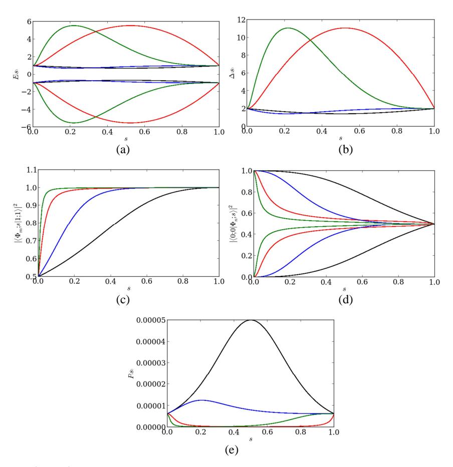
Figure 3 AQC implementation of a Hadamard gate using a linear interpolation function (black line), using a cubic function ( ) 3 2 g s s s s = 3 3 − + (blue line), using extra Hamiltonian = 20 H H e f (red line), using both interpolation function ( ) 3 2 g s s s s = 3 3 − + and extra Hamiltonian = 20 H H e f (green line).

It has been shown that one can use arbitrary interpolation functions, so now we choose a cubic form

\[g(s) = s^3 - 3s^2 + 3s. (39)\]

The result for Hadamard gate without extra Hamiltonian is given in Figure 2; the black line is for linear interpolation and blue line is for cubic interpolation. Because of the non-linear nature of this cubic function, the general effect is a shifting of the curves in the s axis, as expected. Although it does not improve the minimum energy gap, interestingly, it does show a better result for the transition probability between the two states.

The result for AQC implementation of a Hadamard gate with an extra Hamiltonian is given in Figure 3. Similar to the previous figure, the black line is for linear interpolation and the blue line is for cubic interpolation. The red and green lines are for the additional Hamiltonian \(\mathcal{H}_e = 20\mathcal{H}_f\) with linear and cubic interpolation function, respectively. It can be seen that the energy gap, fidelity, mixing probability, and transition probability improve because of the extra Hamiltonian. Similar to the previous results, the role of the cubic function is to shift and deform the curves along the s direction, except for the transition probability.

5 Discussion

We have explored path optimization in AQC for Hadamard gates, given by the Hamiltonian Eq.(17) and Eq.(18). We found that the Hamiltonian path is optimized for f(s) = 1 - g(s) with arbitrary g(s). The extra Hamiltonian will change the energy landscape and, in turn, may change the accomplishment of the adiabatic evolution, either from failure to success or from success to failure. Because h(s) vanishes at the end of the evolution path, it is easy to set h(s) = f(s)g(s) [16], but the choice of the extra Hamiltonian may affect the successfulness of the adiabatic evolution.

The cubic interpolation function seems to give a better result for AQC implementation of the Hadamard gate, as can be seen from Figure 2. It shows some improvement compared to the linear case, especially for the transition probability, which in turn may deliver a speed-up. An even better result can be obtained by combining different approaches in modifying the evolution path.

Adding an extra Hamiltonian does not necessarily give a speed-up, as can be seen from Figure 1(d). It can seen that the mixing probability for k = 5 (red line), k = 10 (blue line), and k = 20 (green line) occur at the end of the evolution, similar to the bare case given by the black line. Nevertheless, we found that an extra Hamiltonian can improve the successfulness of AQC by modifying the energy landscape, i.e. the energy gap is larger for a larger k, as shown in Figure 1(b), and the system will have a greater probability to stay in the ground state, as shown in Figure 1(e). Another result is the change of fidelity as shown by Figure 1(c), either for better or for worse, depending on the extra Hamiltonian. Particularly taking Pauli operator \(\sigma_y\) as the extra Hamiltonian will decrease the fidelity and is harmful to the success of the adiabatic process as well.

6 Conclusion

In conclusion, we have shown that the performance of an adiabatic quantum computation implementation of a single Hadamard gate does not depend on the interpolation functions. Adding an extra Hamiltonian will change the energy landscape, i.e. it may influence the success or failure of the adiabatic evolution, but it does not provide any speed-up. One can choose an arbitrary path, provided that it satisfies the boundary conditions. Nevertheless, a closer look at the evolution of the various parameters reveals other factors that may influence the adiabatic evolution, which should be elucidated in future work.

Appendix

Lagrangian of adding extra Hamiltonian is given by

\[L = -\frac{f(k\dot{h} + \dot{g})}{2|\lambda|^{2}(kh + g)} - \frac{f^{2}\dot{f}}{4|\lambda|^{2}(kh + g)^{2}} + \frac{\dot{f}}{4|\lambda|^{2}} + \frac{\dot{f}}{4(kh + g)^{2}}.\] (40)

After applying the Euler-Lagrange equations, for interpolation function f

\[\frac{\partial L}{\partial \dot{f}} = -\frac{f^{2}}{4|\lambda|^{2}(kh+g)^{2}} + \frac{1}{4|\lambda|^{2}} + \frac{1}{4(kh+g)^{2}} + \frac{1}{4(kh+g)^{2}} + \frac{1}{4|\lambda|^{2}(kh+g)^{2}} + \frac{1}{4|\lambda|^{2}(kh+g)^{2}} + \frac{f^{2}(k\dot{h}+\dot{g})}{2|\lambda|^{3}(kh+g)^{3}} - \frac{k\dot{h}+\dot{g}}{2(kh+g)^{3}} - \frac{f\dot{f}}{2|\lambda|^{2}(kh+g)^{2}} + \frac{f^{2}(k\dot{h}+\dot{g})^{2}}{2|\lambda|^{3}(kh+g)^{2}} + \frac{f^{2}\dot{f}\frac{d|\lambda|}{df}}{2|\lambda|^{3}(kh+g)^{2}} - \frac{\dot{f}\frac{d|\lambda|}{df}}{2|\lambda|^{3}} - \frac{k\dot{h}+\dot{g}}{2|\lambda|^{2}(kh+g)} - \frac{f\dot{f}}{2|\lambda|^{2}(kh+g)^{2}}.\] (41)

The interpolation function g

\[\frac{\partial L}{\partial \dot{g}} = -\frac{f}{2|\lambda|^{2}(kh+g)}\] \[\frac{d}{ds} \left(\frac{\partial L}{\partial \dot{g}}\right) = \frac{f}{|\lambda|^{3}(kh+g)} + \frac{f(k\dot{h}+\dot{g})}{2|\lambda|^{2}(kh+g)^{2}} - \frac{\dot{f}}{2|\lambda|^{2}(kh+g)}, \qquad (43)\] \[\frac{\partial L}{\partial g} = \frac{f(k\dot{h}+\dot{g})\frac{d|\lambda|}{dg}}{|\lambda|^{3}(kh+g)} + \frac{f^{2}\dot{f}\frac{d|\lambda|}{dg}}{2|\lambda|^{3}(kh+g)^{2}} - \frac{\dot{f}\frac{d|\lambda|}{dg}}{2|\lambda|^{3}} + \frac{f(k\dot{h}+\dot{g})}{2|\lambda|^{2}(kh+g)^{2}}\] \[+ \frac{f^{2}\dot{f}}{2|\lambda|^{2}(kh+g)^{3}} - \frac{\dot{f}}{2(kh+g)^{3}}. \qquad (44)\]

For interpolation function h

\[\frac{\partial L}{\partial \dot{h}} = -\frac{kf}{2|\lambda|^{2}(kh+g)}\] \[\frac{d}{ds} \left(\frac{\partial L}{\partial \dot{h}}\right) = \frac{kf}{|\lambda|^{3}(kh+g)} + \frac{kf(k\dot{h}+\dot{g})}{2|\lambda|^{2}(kh+g)^{2}} - \frac{k\dot{f}}{2|\lambda|^{2}(kh+g)}, \tag{45}\] \[\frac{\partial L}{\partial h} = \frac{f(k\dot{h}+\dot{g})\frac{d|\lambda|}{dh}}{|\lambda|^{3}(kh+g)} + \frac{f^{2}\dot{f}\frac{d|\lambda|}{dh}}{2|\lambda|^{3}(kh+g)^{2}} - \frac{\dot{f}\frac{d|\lambda|}{dh}}{2|\lambda|^{3}} + \frac{kf(k\dot{h}+\dot{g})}{2|\lambda|^{2}(kh+g)^{2}}\] \[+ \frac{kf^{2}\dot{f}}{2|\lambda|^{2}(kh+g)^{3}} - \frac{k\dot{f}}{2(kh+g)^{3}}. \tag{46}\]

Differentiating the eigenvalues with respect to s, f, g and h, we get

\[\frac{d|\lambda|}{ds} = \frac{k^2 h\dot{h} + kg\dot{h} + kh\dot{g} + g\dot{g} + f\dot{f}}{|\lambda|},\tag{47}\]

\[\frac{d|\lambda|}{df} = \frac{f}{|\lambda|},\tag{48}\]

\[\frac{d|\lambda|}{dg} = \frac{kh + g}{|\lambda|},\tag{49}\]

\[\frac{d|\lambda|}{dh} = \frac{k(kh+g)}{|\lambda|}. (50)\]

Substititing (47) and (48) into (34) and (35) respectively, we get

\[A(k\dot{h} + \dot{g}) = 0, (51)\] where

\[A = \left[ f^2 + (kh + g)^2 (kh + g)^2 \right]. \tag{52}\]

Substituting (47) and (51) into (43) and (44), and the same procedure for (45) and (46), we get

\[A\dot{f} = 0. \tag{53}\]

Acknowledgments

Suhadi would like to thank Tanoto Foundation for their scholarship, BOPTN for supporting this research, and the members of the Theoretical High Energy Physics Laboratory ITB for their hospitality. FPZ would like to thank ITB and Kemdikbud for their 2013 fiscal year financial support.