
1 Introduction
For the past decades, a thick particle haze that covers the Northern region of Thailand, i.e. Chiang Mai, Chiang Rai, Lamphun, Lampang, Mae Hong Son, Phayao, Phrae and Nan, has been causing serious air pollution problems during the dry season. [1] A haze crisis caused by the dry and stagnant weather conditions occurs every year in the dry season, from February to April, especially in March. These conditions produce dust particles smaller than 10 microns (PM10) suspended in the atmosphere. During this period, a large amount of particulate matters are released into the atmosphere, including carbon monoxide (CO), carbon dioxide (CO2), volatile organic compounds (VOCs), carcinogenic polycyclic aromatic hydrocarbons (PAHs) [2]. The main emission source is biomass open burning, such as forest fires, solid waste burning, and agricultural residue field burning [3,4]. The air pollutants are trapped near ground level due to the meteorological conditions (e.g. stagnant air) and the basin-liked topography surrounded by high mountain ranges results in restricted pollution dispersion. In addition, low rainfall in dry season effect on violence of haze problem. For this reason, the leaching of smoke or dust particles in the air is low [4]. A report from the Pollution Control Department revealed that Chiang Mai province encounters ever longer and more serious smog problems.
During haze periods, the 24-hour average concentrations of particulate matter with an aerodynamic diameter smaller than 10 micron (PM10) frequently exceed the Thailand National Ambient Air Quality Standard (NAAQS) of 120 micron [5]. Also, the Public Health Ministry of Thailand [1] has reported an increase in bronchial asthma and respiratory diseases in people living in these areas. In addition, these fine particles contain carcinogenic polycyclic aromatic hydrocarbons that can induce lung cancer [6]. The smoke haze episodes affect not only adverse health problems but also reduce visibility and cause economic sectors to decline, i.e. tourism, transportation, and agriculture. Therefore, the Thai government shows increasing concern to get the smoke haze problem under control [5].
The PM10 measurement method is complex and it takes a long time to analyze the results with a performance tool [7]. In order to simplify this process, we utilized a logistic regression analysis method for establishing the occurrence of haze. As the first step, we determined the main factors associated with the occurrence of haze in the Chiang Mai area. The second step was to establish a mathematical model to represent the occurrence of haze using the main factors from the logistic regression analysis. Lastly, we used the mathematical model to predict the occurrence of haze in the next year. This study can be used as guidance for monitoring haze problems in the northern region of Thailand.
2 Study Data
This study is based on an investigation of hourly measured data over a six-year period, from 2005 to 2010. PM10 is one of five air pollutants that are used to measure air quality in Thailand. The Air Quality Index (AQI) is a number used by government agencies to communicate to the public how polluted the air is currently or how polluted it is forecasted to become.
2.1 Air Quality Index
The Air Quality Index (AQI) is an indicator of air quality, based on air pollutants that have adverse effects on human health and the environment. The main pollutants for Thailand are: O<sub>3</sub>, SO<sub>2</sub>, NO<sub>2</sub>, CO and PM<sub>10</sub>. The maximum AQI from these five pollutants is an indicator of the air quality for a particular day or moment. The Pollution Control Department of the Ministry of Natural Resources and Environment is the organization in Thailand that measures the AQI and reports the results [8,9].
The effects of air pollution on people's health can become a cause for concern, as shown Table 1. During the dry season of 2007, there was no rainfall for 6 months (November 2006 - April 2007). The occurrence of smoke haze affected a high \(PM_{10}\) concentration of up to 303.9 micron [4]. The number of patients infected with respiratory diseases and allergies increased dramatically according to a report from the Public Health Department of Chiang Mai province.
AOI Level of Health Colors Meaning Values Concern Air quality is considered satisfactory, 0 - 50Blue Good and air pollution poses little or no risk. Air quality is acceptable; however, for some pollutants there may be a 51-100 Moderate Green moderate health concern for a very small number of people who are unusually sensitive to air pollution. Members of sensitive groups may 101-200 Unhealthy Yellow experience health effects. The general public is not likely to be affected. Everyone may begin to experience 201-300 Very unhealthy health effects: members of sensitive Orange groups may experience more serious health effects. Over Health alert: everyone may experience Red Hazardous 300 more serious health effects.
Table 1 Air Quality Index criteria in Thailand.
Source: Pollution Control Department (www.pcd.go.th)
\(2.2 PM_{10}\)
\(PM_{10}\) is suggested as an indicator with relevance to the majority of the epidemiological data. It is extensively measured throughout the world [10,11]. As mentioned earlier, knowing the occurrence of \(PM_{10}\) from the ambient parameters is significantly necessary. The standard level of \(PM_{10}\) in Thailand is declared at 120 micron. However, during haze occurrence, 100 micron is set to monitor and alert people. In this study, PM10 was investigated in order to categorize haze occurrence response into 3 levels (0, 1 and 2) using logistic regression analysis. The detection limits were 0-99, 100-119, and over 120 micron, respectively indicating: little health effect; more health effect and alert; more serious health effect. PM10 was implicated with associated factors for predicting the occurrence of haze.
3 Methodology
The procedure of this research was as follows:
- Step 1: Collect data of PM10, CO, NO, NO2, SO2, O3, wind direction, temperature, relative humidity (RH), pressure, wind speed and rainfall.
- Step 2: Find the relationships between PM10 and others parameters by Pearson correlations for relationship classification into high, moderate, or low.
- Step 3: Construct logistic regression for haze problem model using high and moderate relationships. Define response function on the basis of PM10 concentrations, reflecting the different ranges as: "little health effect (0-99)", "more health effect and alert (100-119)" and "more serious health effect (over 120)".
- Step 4: Analysis and discussion of logistic regression model. Present goodness of fit by Pseudo R2 .
- Step 5: Consider level of health concern for PM10 levels in 2011 to indicate health effects.
3.1 Logistic Regression Analysis
Logistic regression or logit regression is a type of regression analysis used for predicting the outcome of a categorical dependent variable based on one or more predictor variables. That is, it is used for estimating the empirical values of parameters in a qualitative response model. The probabilities describing the possible outcomes of a single trial are modeled as a function of the predictor variables using a logistic function. Usually, logistic regression is used to refer specifically to problems in which the dependent variable is binary, which means that the number of available categories is two. Problems with more than two categories are referred to as multinomial logistic regressions or, if the multiple categories are ordered, as ordered logistic regressions [12,13]. Moreover, logistic regression measures the relationship between a categorical dependent variable and one or more independent variables that are usually continuous. The probability scores are utilized as the predicted values of the dependent variable [14].
3.2 Mathematical Model
Haze smoke problems normally occur in Northern Thailand for a short period from February to April each year, peaking in March. The factors relating to this problem correspond to 11 parameters [9,12], i.e. PM<sub>10</sub>, CO, NO, NO<sub>2</sub>, SO<sub>2</sub>, O<sub>3</sub>, wind direction, temperature, relative humidity (RH), pressure, wind speed, and rainfall. In order to identify the relationships between PM<sub>10</sub> and the others parameters, the Pearson correlations were analyzed.
3.2.1 Model Formulation
The objective of modeling the relation between the occurrence of haze (dependent variable) and concentrations of gases with meteorological data (independent variables) is to estimate the probability of the former given the incidence of the latter. An explanation of logistic regression begins with an explanation of the logistic response function, which always takes on values between zero and one. Let \(P_i\) denote the multinomial probability of an observation falling in the j th category. Category j is used as the base level of the method (any category can be taken as the base level). We want to find the relationship between this probability and n explanatory variables, \(x_1, x_2, ..., x_n\). The multinomial logistic regression model then is
\[\ln(P_i/P_j) = \beta_{0i} + \beta_{1i}x_1 + \dots + \beta_{ni}x_n \tag{1}\] and \[P_1 + P_2 + ... + P_j = 1\] (2)
where \(\beta_0, \beta_1, ..., \beta_n\) are model parameters for i = 1, 2, ..., m.
Since all the P's add to unity, this can be reduced to
\[P_{i} = \frac{\exp(\beta_{0i} + \beta_{1i}x_{1} + \dots + \beta_{ni}x_{n})}{1 + \sum_{k=1}^{j-1} \beta_{0k} + \beta_{1k}x_{1} + \dots + \beta_{nk}x_{n}}\](3)
For i = 1, 2, ..., j - 1
\[P_{j} = \frac{1}{1 + \sum_{k=1}^{j-1} \beta_{0k} + \beta_{1k} x_{1} + \dots + \beta_{nk} x_{n}}\](4)
The model parameters are estimated by the method of maximum likelihood [12,13].
3.2.2 Estimation of Model Parameters in Logistic Regression
The regression coefficients are usually estimated through an iterative maximum likelihood method. Unlike linear regression with normally distributed residuals, it is not possible to find a closed-form expression for the coefficient values that maximizes the likelihood function, so an iterative process must be used instead [13].
The log likelihood functions for the multinomial logistic regression model are:
\[\ln L = \sum_{i=1}^{N} \sum_{r=1}^{j-1} \left( y_{ir} \sum_{k=0}^{K} \beta_{kr} x_{ik} - n_i \ln \left( 1 + \sum_{r=1}^{j-1} \exp \left( \sum_{k=0}^{K} \beta_{kr} x_{ik} \right) \right) \right)\] (5)
where \(Y_{ir}\) is a known, fixed constant value. Logistic regression models require a minimum of log likelihood to find parameters \(\beta_0, \beta_1, ..., \beta_n\). Since Eq. (5) is nonlinear, Newton's method is used for this model. [14]
3.2.3 Measurement of Relationships
In linear regression, the squared multiple correlation \(R^2\) is used to assess goodness of fit, as it represents the proportion of variance in the criterion that is explained by the predictors. In logistic regression analysis, there is no agreed upon analogous measure but there are several competing measures, each with its own limitations [12]. Pseudo \(R^2\) is used to assess goodness of fit, as it represents the proportion of variance in the criterion that is explained by the predictors in the logistic regression analysis. The Pseudo \(R^2\) formula used here is:
\[Pseudo R^{2} = \frac{-2\log L_{Null} - \left[2\log L_{Model}\right]}{-2\log L_{Null}}\] (6)
where \(L_{\it Null}\) is a likelihood function with only constants \(L_{\it Model}\) is a likelihood function with the predicted value defined
Pseudo R<sup>2</sup> always takes on values between zero and one.
4 Results and Discussion
\(PM_{10}\) is an important variable that indicates the violence of a haze situation. In this study, we firstly found the correlation coefficient between \(PM_{10}\) and the concentrations of gases along with meteorological factors to formulate a model for predicting the occurrence of haze using a logit function.
4.1 Results of Correlation Coefficients
Correlation analysis was used to approach the relationship between two or more variables by correlation coefficient (r) values from –1 to 1. A negative value represents a contrary relationship, whereas a positive value shows the same direction among the sets of variables [12]. The values were defined as follows: (i) r from 0.50 to 1.00 or from –0.50 to –1.00 was considered a high correlation; (ii) from 0.30 to 0.49 or –0.30 to –0.49 was considered a moderate correlation; (iii) from 0.10 to 0.29 or –0.10 to –0.29 was considered a low correlation; and (iv) zero represents no relationship.
From the above principle, we obtained seven main factors associated with the concentration of PM10, derived from the high and moderate correlation values, as shown in Table 2. Thus, the main factors associated with the PM10 concentration are CO, NO2, O3, RH, SO2, NO and pressure. We tried using only the high correlation group, which resulted in less accuracy than using both the high and moderate correlations.
| Factors | Correlation | Factors | Correlation |
|---|---|---|---|
| CO | 0.6676 | Temperature | 0.0160 |
| NO | 0.3191 | RH | -0.6633 |
| NO2 | 0.8245 | Pressure | 0.3278 |
| SO2 | 0.4719 | Wind Speed | -0.0642 |
| O3 | 0.5576 | Wind Direction | -0.0865 |
| Rainfall | -0.2234 |
Table 2 Correlation coefficients of all parameters.
In contrast to the independent variables (Xi), which are quantitative variables, the dependent variable (Y) is a qualitative variable. Moreover, the values of Y were coded for the smog problems into 3 cases. The response function on the basis of PM10 concentrations reflects the different ranges as shown in Table 2 , where all the values of CO, NO2, O3, RH, SO2, NO are in g/m3and pressure is in bar.
Let P1 be the probability that 0 PM10 99, or, "little health effect"; P2is the probability that 100 PM10 119, or, "more health effect and alert"; and P3 is the probability that PM10 120, or, "more serious health effect". Category 1 is the base level in our description of the method.
The logistic regression models of this study are:
\[\ln(P_2/P_1) = \beta_{02} + \beta_{12}x_1 + \dots + \beta_{72}x_7 \tag{7}\]
\[\ln(P_3/P_1) = \beta_{03} + \beta_{13}x_1 + \dots + \beta_{73}x_7 \tag{8}\] and \(P_1 + P_2 + P_3 = 1\)
This can be reduced to:
\[P_{1} = \frac{1}{1 + \sum_{k=2}^{3} \beta_{0k} + \beta_{1k} x_{1} + \dots + \beta_{7k} x_{7}}\] \[(9)\]
\[P_{2} = \frac{\exp(\beta_{02} + \beta_{12}x_{1} + \dots + \beta_{72}x_{7})}{1 + \sum_{k=2}^{3} \beta_{0k} + \beta_{1k}x_{1} + \dots + \beta_{7k}x_{7}}\](10)
and \[P_3 = \frac{\exp(\beta_{03} + \beta_{13}x_1 + \dots + \beta_{73}x_7)}{1 + \sum_{k=2}^{3} \beta_{0k} + \beta_{1k}x_1 + \dots + \beta_{7k}x_7}\] (11)
where \(x_1, x_2, ..., x_7\) are concentration of CO, NO<sub>2</sub>, O<sub>3</sub>, RH, SO<sub>2</sub>, pressure and NO, respectively.
4.2 Results of Coefficient Estimation
The logistic regression models are
\[\ln(P_2/P_1) = 0.896x_1 + 0.205x_2 - 0.052x_3 + 0.068x_4 + 0.113x_5\]\[-0.114x_6 + 0.256x_7 - 89.639 \tag{12}\]
\[\ln(P_3/P_1) = 2.232x_1 + 0.362x_2 - 0.103x_3 + 0.136x_4 + 0.242x_5\]\[-0.136x_6 - 0.06x_7 - 188.344 \tag{13}\]
Considering the seven predictive variables that influence the occurrence of smog derived from \(PM_{10}\) concentration and considering the predictive ability of the logistic model, the variation of this haze problem model is 59.6% (Pseudo \(R^2 = 0.5960\)). The accuracy of the model was 94.66%.
Figure 1 shows the multinomial logistic regression of this model for 2011. The accuracy of the model for 2011 was 92.33%. Figure 2 shows when high concentrations of PM<sub>10</sub> affecting the haze situation advise monitoring and forecasting of criteria pollutants in the air during March and April in 2011. From the smog haze prediction for 2011 it can be seen that it is an important task to make how bad or good the air quality is for human health easily
understandable and to assist in data interpretation for the decision making processes related to pollution migration measures and air quality management.
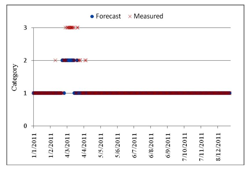
Figure 1 Multinomial logistic regression model in 2011.
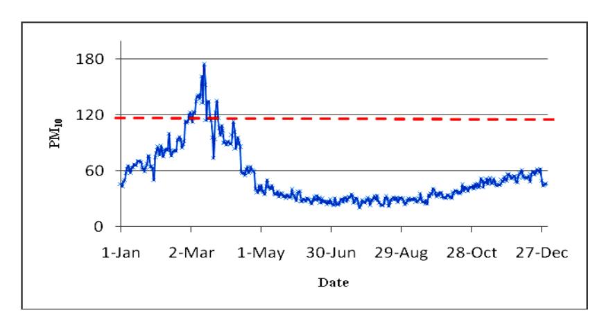
Figure 2 Plot of PM10daily concentrations from PCD, Thailand in 2011.
Figure 3 shows that smog haze situations affecting the level of human health concerns could be classified into 3 levels of air quality: "Good" about 60% (219/365), "Moderate" about 31.23% (114/365), and "Unhealthy" about 8.77% (32/365). A comparison between the observed values and the model's predicted values suggests that the model can be used for the prediction of daily PM10 concentrations in urban areas.
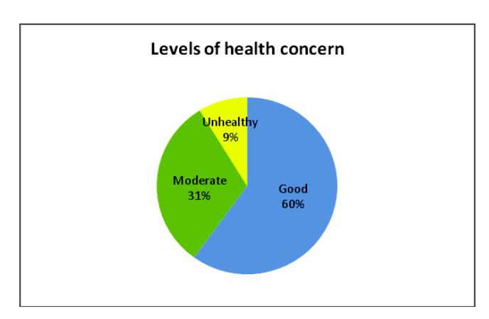
Figure 3 Level of Health Concern of PM10 in 2011.
5 Conclusions
A modeling effort was conducted in order to investigate human health concerns related to smoke haze for decision-making purposes. Logistic regression analysis was used as a tool for achieving the difficult task of predicting daily PM10 concentrations based on the main parameters affecting smog haze situations in Chiang Mai province. As a result it is believed that the derivation of PM10 concentrations from the parameters affecting smog haze situations should be considered as a tool for operational use in PM10 concentration forecasting, aiding the protection of the exposed population against short-term variations in particulate matter levels.
Acknowledgements
The authors would like to thank the Pollution Control Department in Thailand, which kindly provided valuable data. The financial support for this research project from the faculty of Science, King Mongkut's Institute of Technology Ladkrabang, Thailand is gratefully acknowledged.