
1 Introduction
On 6 March 2007, two earthquakes occurred at about 10:50 and 12:50 (local time) along two major segments of the Sumatran fault near Singkarak Lake in western Sumatra, Indonesia (Figure 1). The National Earthquake Information Center (NEIC)-United States Geological Survey (USGS) reported these events as southern earthquakes with Mw 6.4 at 0.512°S, 100.524°E and Mw 6.3 at 0.49°S, 100.52°E. The epicenters were approximately 50 km from Padang, the capital city of West Sumatra. Strike, dip and rake of both events are 150°, 85° and -176°, respectively. We refer to these quakes as the Singkarak earthquakes because the position of the Singkarak Lake is in between both epicenters. The two quakes destroyed structures on or near the fault, killing more than 70 inhabitants. These events were intraplate earthquakes along the Sumani (Figure 2) and Sianok (Figure 3) segments as parts of the Sumatra fault. This fault accommodates the strike-slip component of the oblique convergence of the subduction of the Indian and Australian plates under the Sumatran Island. The dip slip component is accommodated on the subduction zone [1-2].
Because these events were shallow quakes, the surface displacements can be investigated directly. Natawidjaja, et al. [3] reported that the total length of surface rupture of the first event was up to 15 km with a surface displacement from a few centimeters to 24 cm right lateral along the Sumani segment (Figure 2). The second one had a length of about 22 km and the surface displacement was only up to 12 cm along the Sianok segment (Figure 3). The fault slips of both events seemed to diminish toward both ends.
The events were recorded by many seismometers distributed all over the world and collected by the Global Seismological Network (Incorporated Research Institutions for Seismology [IRIS]/USGS, International Deployment for Accelerometers [IRIS]/IDA). In this research, we investigated the source processes of both events using teleseismic data and applying the slip inversion method of Yoshida, et al. [4].
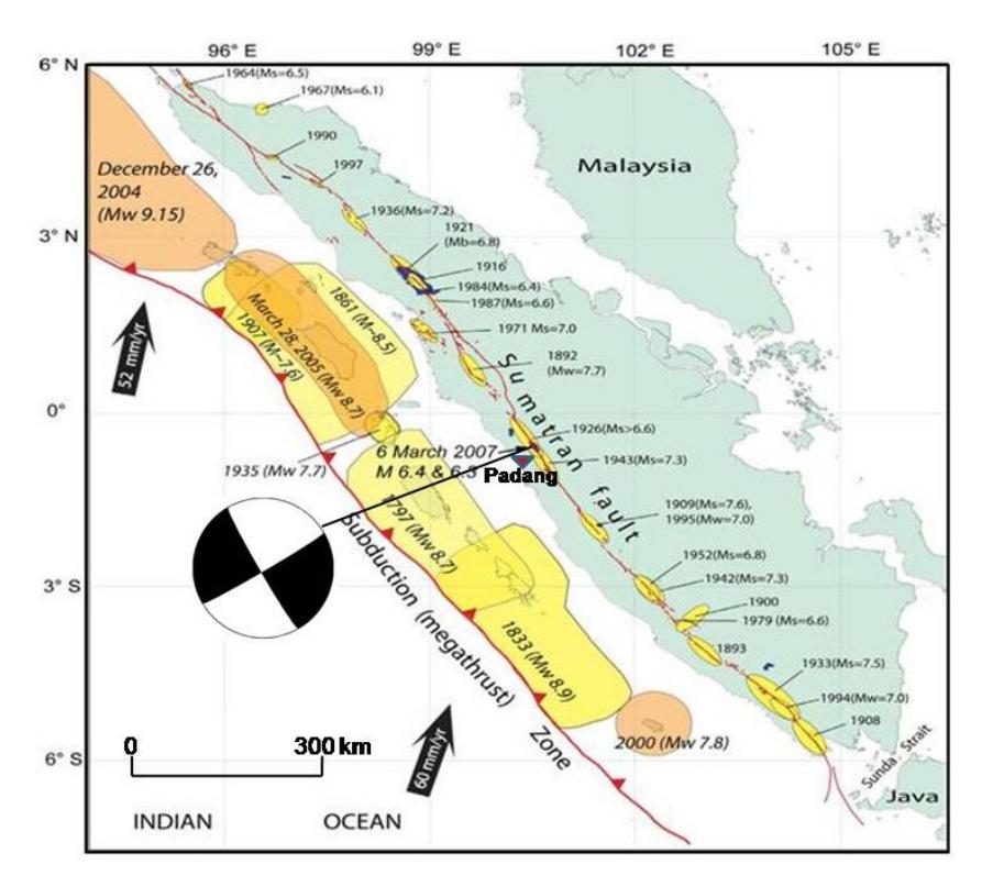
Figure 1 Historical major earthquakes along the Sumatran fault zone (SFZ) since 1892, including the 6 March 2007 events. The ellipsoid shapes indicate fault segments that were ruptured. The large ellipsoids west of Sumatra indicate recent and historical megathrust events in the Sumatra subduction zone.
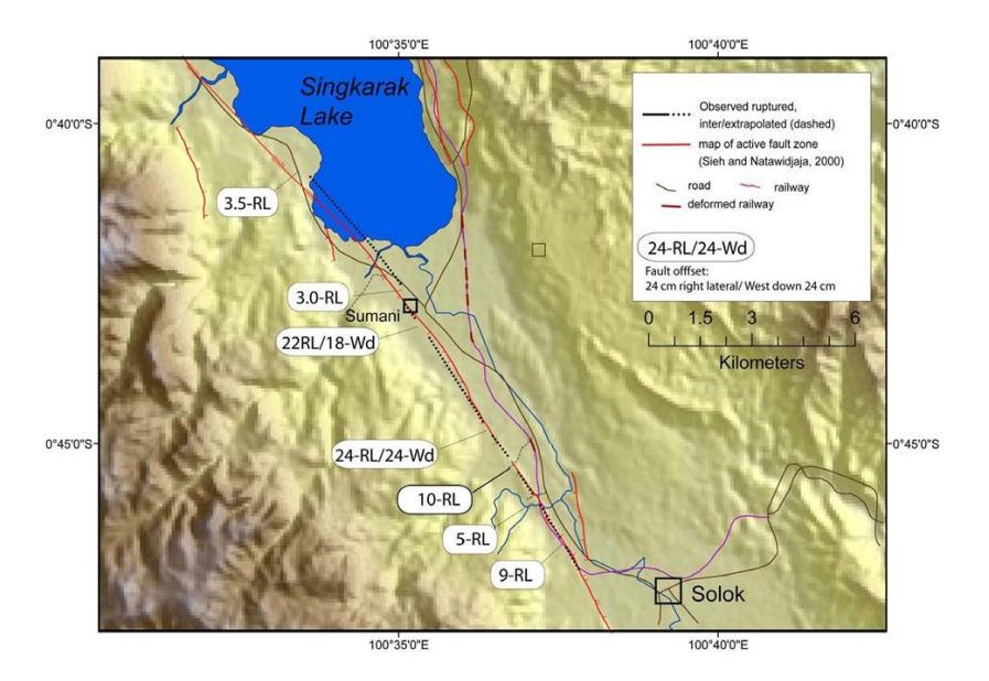
Figure 2 Surface fault displacements and measured fault offsets of the first main-shock. The length of the surface rupture zone was up to 15 km. The offsets varied from a few cm up to 24 cm displacement (west side down) of right-lateral movements. The largest slip occurred at the central part of the rupture. The dipslip movements were also observed [3].
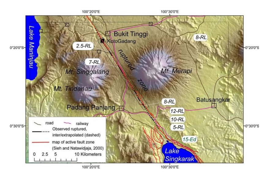
Figure 3 Surface fault ruptures and fault offsets of the second mainshock. The length of the rupture zone was up to 22 km. The largest slip, up to 12 cm, occurred at the central part of the rupture [3].
2 Teleseismic Data
We used the vertical component of P waves and transverse component of S waves picked from teleseismic velocity seismograms. The waveform data were filtered spatially with station-epicenter distance ∆>30° to avoid triplication effects and ∆<100° to avoid wave diffraction. The station distribution in this distance range is shown in Figure 4.
Seismograms were deconvolved from instrument response, integrated to obtain the ground displacements, filtered temporarily with bandpass from 0.02 to 0.4 Hz and resampled at a rate of 1.0 s. The duration for the inverted waveform was 60 seconds, picked from the onsets of P- and S-waves. These processes were execute using the SAC2000 program [5].
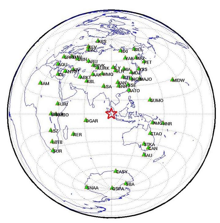
Figure 4 Distribution of teleseismic stations with station-epicenter distance between 30° and 100°. The star symbol is for the two epicenters.
3 Slip Inversion Method
We applied the slip inversion method from Yoshida, et al. [4] to the teleseismic data. We define the fault parameters as listed in Table 1, based on the focal mechanism from NEIC-USGS explained in the introduction and the surface
displacement data (Figures 2 and 3). NEIC-USGS released two-conjugate fault planes: (150°,85°,-176°) and (60°,86°,-5°). We chose the first, because the strike coincided with the surface lineation. As shown in Figure 5, the epicenters were assumed to coincide with the largest surface displacements with a depth of 15 km and the fault line coincided with the Sumani and Sianok segments.
| Table 1 | Source parameters. |
|---|
| Parameters | |
|---|---|
| Origin time | 03:49:39 (first event) |
| 05:49:27 (second event) | |
| Hypocenter | 0.75°S, 100.6°E, 15 km (first event) |
| 0.48°S, 100.5°E, 15 km (second event) | |
| Strike, dip, rake | 150º, 85º, -176º |
| Fault length | 36 km |
| Fault width | 16 km |
| Number of subfaults | 9 x 4 |
Figure 5 Locations of the epicenters and fault length based on the largest surface displacement (Figures 2 and 3) and segmented faults.
The fault length along the strike direction was 36 km and its width was estimated by rule of thumb to be about 16 km, i.e. 0.4 of its length (Leonard, 2010 [6]). The fault plane was divided into 9×4 subfaults with a grid size of 4 km and the slip was made variable at each subfault. The point dislocation was approximated at the center of each subfault. The 10 s time function of dislocation was expressed by a superposition of several ramp functions with rise time τ=1 s, and the interval of adjacent functions was assumed to be equal to τ.
The rupture time \(T_{mn}\), which is the time when the rupture front reached the center \((x_m, y_n)\) of the mn-th subfault was defined as
\[T_{mn} = \sqrt{x_m^2 + y_n^2} / V_r \,, \tag{1}\] where \(V_r\) is the rupture velocity. In this case, we applied \(V_r = 2.5 \, \mathrm{km/s}\) obtained from general rule of thumb (about 0.8 of S-wave velocity at the fault). The slip vector on the subfault is represented by a linear combination of two components in the direction \(\lambda^0 \pm \pi/4\), where \(\lambda^0\) is the initial rake angle (176° in this case). Each component of the mn-th subfault was further divided into l elements \(X_{mnl}\) or \(Y_{mnl}\) which denote slips during \(T_{mn} + (l-1)\tau < t < T_{mn} + l\tau\).
Letting k = 1 and 2 be P and SH wave components, respectively, the synthetic seismograms at station \(\mathbf{x}_i\) from the source model was calculated as
\[F_{k}(t_{i}, \mathbf{x}_{j}) = \sum_{mn} X_{mnl} f_{mnk}(t_{i} - (l-1)\tau - T_{mn}, \mathbf{x}_{j})\] \[+ \sum_{mn} Y_{mnl} g_{mnk}(t_{i} - (l-1)\tau - T_{mn}, \mathbf{x}_{j})\] (1)
where \(f_{mnk}\) and \(g_{mnk}\) are the k-th components of the seismic Green's function for the mn-th subfault with unit slip in the direction \(\lambda^0 \pm \pi/4\). They were calculated by a ray theory with isotropic PREM with attenuation time constant \((t^*)\) of 1 s for the P-wave and 4 s for the SH-wave.
To avoid instability of the inversion problem, we applied smoothing and positivity constraints on the slip distribution. The Laplacian operator was defined as
\[\nabla^2 X_{m,n,l} = X_{m+1,n,l} + X_{m,n+1,l} + X_{m,n,l+1} - 6X_{m,n,l} + X_{m-1,n,l} + X_{m,n-1,l} + X_{m,n,l-1}\] and
\[\nabla^2 Y_{m,n,l} = Y_{m+1,n,l} + Y_{m,n+1,l} + Y_{m,n,l+1} - 6Y_{m,n,l} + Y_{m-1,n,l} + Y_{m,n-1,l} + Y_{m,n,l-1}\] were used as smoothing constraints. The components of slips \(X_{mnl}\) and \(Y_{mnl}\) were always positive, which can be expressed as penalty functions \(1/\sqrt{X_{mnl}}\), \(1/\sqrt{Y_{mnl}}\), which can increase to infinity as \(X_{mnl}\) and \(Y_{mnl}\) approach zero. The strength of those constraints was determined by the ABIC method [4].
4 Slip Inversion Results and Discussion
The slip inversion results show that the first event had three asperities (Figure 6). They were 1.5 m at the shallow side, 0.7 m at the south-east deep side, and 0.5 m at the north-west deep side. The largest one was responsible for the larger surface displacements around the epicenter area (Figure 2). This event released a total seismic moment of \(7.9 \times 10^{18}\) Nm (Mw 6.5) using a rigidity of \(3 \times 10^{11}\) Nm<sup>-2</sup>. The seismograms were well recovered as shown in Figure 7. Although there was some variance below 0.55, the main patterns were still well recovered. The slip rate function at each subfault shown in Figure 8 indicate that the inversion result is reasonable because a decreasing pattern of displacement after the maximum displacement occurred.
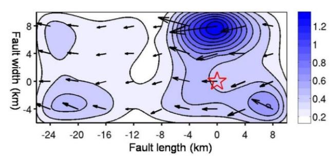
Figure 6 Total slip distribution (in meter) of the first event.
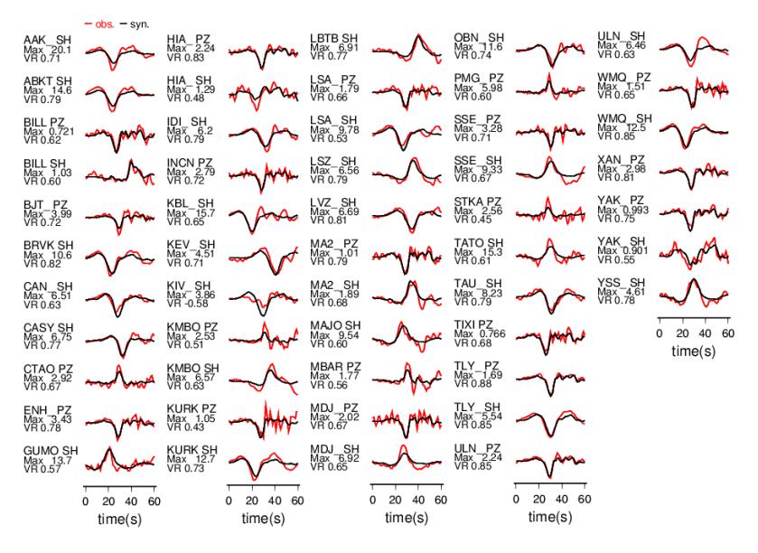
Figure 7 Comparison of observed (red) and calculated (black) teleseismic displacement waveforms of first events. Maximum amplitude (Max) in \(\mu\)m and variance reduction (VR) are given to the left of each waveform.
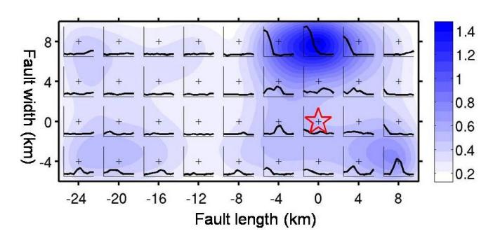
Figure 8 Slip rate function (in meters) at each subfault of the first event. The crosses denote the location of the point sources in the subfaults.
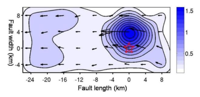
Figure 9 Total slip distribution (in meter) of the second event.
The inversion result of the second event has one asperity and released 7.5×10¹⁸ Nm (Mw 6.5) (Figure 9). Although, the first event released a larger energy, the maximum slip of the first event (1.5 m) was smaller than that of the second event (1.7 m). This means that the energy of the second event was concentrated at its asperity. This asperity was responsible for the larger surface displacements around the epicenter area (Figure 3). This event can be treated as a point source. The good data fit and the reasonable patterns of time slip rate are shown in Figures 10 and 11.
We can note the specific characters of the two events. Firstly, the slip rate history of the shallow parts of the large asperities in Figure 8 and 11 have specific characters that start with large slips and decrease rapidly. The deep parts show that the slip starts with smaller values, then increases to maximum and decreases again. Secondly, the resultant slip distribution shows that the largest asperity area of both events was located shallower than the hypocenter. These features may have been caused by the brittle condition as a function of the depth of the material around the fault planes. This should be investigated using a method such as regional tomography.
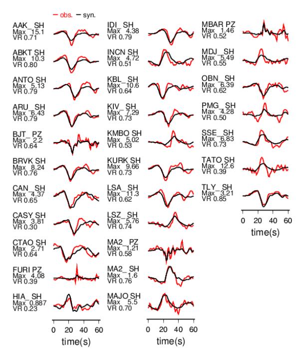
Figure 10 Comparison of observed (red) and calculated (black) teleseismic displacement waveforms of second events. Maximum amplitude (Max) in μm and variance reduction (VR) are given to the left of each waveform.
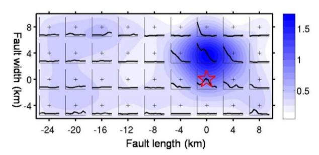
Figure 11 Slip rate function (in meters) at each subfault of the second event. The crosses denote the location of the point sources in the subfaults. The star shows the hypocenter.
5 Conclusion
We have studied the source processes of the Singkarak earthquakes using teleseismic data. The first event had three asperities with a maximum slip of 1.4 m and it released a total seismic moment of 7.9×10¹⁸ Nm (Mw 6.5), while the second event had one asperity with a maximum slip of 1.7 m and it released a seismic moment of 7.5×10¹⁸ Nm (Mw 6.5). Both maximum slips occurred above the hypocenters and were responsible for the surface displacement patterns.
Acknowledgements
This research was funded, Bandung Institute of Technology, Bandung, Indonesia, under by International Research No. 150a/K01.08/SPK/2009. The figures were drawn using the Genetic Mapping Tools [7].