
1 Introduction
One method used to estimate the amount of rainfall through the infrared (IR) channel of weather satellites is the convective stratiform technique (CST) [1-5]. According to Levizzani, et al., [6] and Kimani [7], this method can be categorized as a cloud model technique. It considers cloud physics, while the estimation process utilizes only infrared weather satellite data. Based on previous studies, CST is considered to have the best performance compared to other infrared methods [1].This method has also shown good results when applied in Indonesia [5]. However, the IR data utilized in CST are reported to have a number of limitations, such as having a weak interaction and low
Received June 28th, 2013, 1 st Revision May 12th , 2014, 2nd Revision June 4th , 2014, 3rd Revision August 20th 2014, Accepted for publication August 26th, 2014.
Copyright © 2014 Published by ITB Journal Publisher, ISSN: 2337-5760, DOI: 10.5614/j.math.fund.sci.2014.46.3.4
sensitivity to hydrometeors. This is due to the infrared data's lack of a strong physical connection between the remotely sensed signal and surface rainfall. They correspond only to cloud top brightness temperature, which is indirectly related to surface rainfall [8-10]. This condition can affect the performance of CST in estimating rainfall. However, these limitations can be overcome by, alternatively, utilizing passive microwave (PMW) data. These data also have limitations, in time and spatial resolution, but they are better than IR in detecting hydrometeors and there is a strong connection between the remotely sensed signal and surface rainfall [9,11,12]. As the two types of data potentially complement each other, combining PMW and IR data is another alternative solution for improving the quality of the estimation result [9,11-14].
The objective of this study was to estimate rainfall using a modified CST, called CSTm, created by applying a variability index (VI) that leverages PMW data. The VI separates convective and stratiform rainfall in CSTm using PMW data, replacing the role of the slope parameter (S) in CST, which uses IR data. The fact that the implementation of PMW data results in a wider scope of the average covered area was considered.
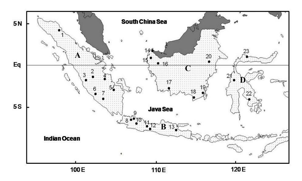
Figure 1 Distribution of rainfall observation points on the islands of Sumatra (A), Java (B), Kalimantan (C) and Sulawesi (D).
Due to the limited availability of PMW data, the rainfall estimation in this study was only done on IR and PMW data obtained at the same or at adjacent observation times and from the same area. The IR data were available for every hour or 24 times a day and always covered the same area, while the PMW data were available only twice a day (every 12 hours) and did not always cover the same area. Therefore, in general, there were two sets of data that relatively coincided daily. The utilization of both IR and PMW data was expected to improve the ability of the modified CST to correctly estimate rainfall. To verify the results, the estimated rainfall values were compared with real observation data that were available from 23 observation points spread over the four major islands in Indonesia, as shown in Figure 1.
2 Modification of CST
2.1 The Original Form of CST
The original form of CST used in this study applies rainfall estimation steps similar to the procedures proposed by Adler and Negri [1], Goldenberg, et al. [2] and Islam, et al. [4]. The estimation actions include, among others, the application of techniques to identify convective cores and their locations, utilizing IR imagery from geostationary meteorological satellites (GMS), and determination of the intensity of convective and stratiform rain. The calculations of other precipitation components in the estimation process were still used in this study. GMS imagery as the IR data source in this study was replaced by multi-functional transport satellite (MTSAT) 1R imagery, as the GMS was no longer working. To identify the location of convective cores, an examination was conducted toward the equivalent infrared blackbody temperature (\(T_{BB}\)) to find \(T_{min}\). After the pixel location of \(T_{min}\) was identified, its strength was measured by calculating the slope parameter (S), which is shown by:
\[S = k \left( T_{i-1,j} + T_{i+1,j} + T_{i,j-1} + T_{i,j+1} - 4T_{i,j} \right)\] (1)
where i and j refer to the position of the pixel for which S is calculated, while the factor k=0.25 is a value that depends on the amount of surrounding data that are taken into account. In this study, the slope parameter (S) was calculated by considering the eight surrounding pixels, so k became 0.125 [5]. For this purpose, Eq. (1) was rewritten as follows:
\[S = k \left( T_{i-1,j-1} + T_{i-1,j} + T_{i+1,j} + T_{i+1,j+1} + T_{i,j+1} + T_{i-1,j+1} + T_{i-1,j+1} + T_{i-1,j+1} + T_{i+1,j-1} - 8T_{i,j} \right)\] (2)
According to Goldenberg, et al., [2], to distinguish convective cores at the identified location, the criteria as shown by Eq. (3) should be fulfilled:
\[S \ge \exp \left[ 0.0826 \left( T_{\min} - 207 \right) \right]\] (3)
The convective precipitation area \((A_c)\), according to Adler and Negri [1], is directly related to cell top height as indicated by the cloud top temperature \((T_{min})\). The \(A_c\) is determined by the following formula:
\[1 \quad (A_c) = a T_c + b \tag{4}\] where a = -0.0492 and b = 15.27 are constants that were calculated by Adler and Negri [1] for FACE (Florida Area Cumulus Experiment) and by Goldenberg, et al. [2] for WMONEX (Winter Monsoon Experiment). The term \(T_{min}\) in Eq. (3) is then replaced by \(T_{ci}\), where index i refers to the i-th core.
In the original CST, there is a separation step necessary to determine convective or stratiform rainfall. The calculations for convective and stratiform rainfall are different, depending on the results of a comparison between the slope parameter (S) and the identified \(T_{min}\), as shown in Eq. (3). Islam, et al. [4] proposed to calculate convective and stratiform rainfall as follows:
Convective rainfall \[(mm) = c (A_c / A) TR_c\] (5)
Stratiform rainfall \[(mm) = s(A_s / A)TR_s\] (6)
where c = number of convective cells within a grid, s = number of stratiform cells within a grid, \(A_c\) = convective rain area from Eq. (4), \(A_s\) = stratiform rain area in that grid, A = average area covered by each pixel, T = length of period in hour, \(R_c\) = convective rain rate in mm h<sup>-1</sup> (20 mm h<sup>-1</sup>) [4], \(R_s\) = stratiform rain rate in mm h<sup>-1</sup> (3.5 mm h<sup>-1</sup>) [4].
2.2 Modifications
In the separation of the convective and stratiform portions in the algorithm steps of CST, the modification of CST to become CSTm was started by replacing the slope parameter (S), which uses IR data, with the variability index (VI), which uses PMW data. If the value of S shown in Eqs. (1), (2) and (3) is equal to or higher than the threshold, the separation result will show the convective portion, and otherwise, it will show the stratiform portion. In the modified CST, Eqs. (1), (2) and (3) – the algorithm steps that calculate the value of S— are replaced by the VI, while Eqs. (4) to (6) of the same steps are still used in CSTm. Therefore, the VI is only used in CSTm to separate the convective from the stratiform portion in the algorithm steps and not to determine the estimated rainfall value. In CSTm, the VI utilizes PMW data instead of IR data, as they have a better interaction with the hydrometeors. Thus, it was expected that the separation result using the VI would be more accurate and would have a significant contribution in improving the quality of the estimation results.
Anagnostou and Kummerow [15] define the determination of the value of VI in the separation process that utilizes PMW data as follows:
\[VI = \frac{1}{N} \sum |X_i - X_0| \tag{7}\]
Where \(X_0\) is the value of the central pixel, \(X_i\) denotes the values of the surrounding pixels, and N is the total number of surrounding pixels used. The value X can be any observed quantity related to rainfall; in this study X was replaced by the satellite brightness temperature. Determination of the stratiform and convective portions based on the VI value is shown in Table 1[15], which displays the probabilistic relationship between the stratiform coverage over the view of the satellite field and horizontal polarization of mean absolute 85-GHz brightness temperature. This study, however, used a brightness temperature of 89 GHz due to the limited data available in the Advanced Microwave Sounding Unit (AMSU) B. Based on the data in Table 1, the convective portion is determined if the VI threshold value is higher than 8, where the occurrence probability of stratiform coverage exceeding 70 percent is only 0.44. This probability value becomes smaller if the threshold value is higher than 8. If the VI threshold value reaches 8 or lower, then the stratiform portion is determined.
Table 1 Classification scheme – probability of stratiform coverage occurrence.
| Stra | atiform coverage ( | %) | |||
|---|---|---|---|---|---|
| VI | >70 % | 40% - 70% | < 40% | ||
| Probability of occurrence | |||||
| 0 – 8 | 0.67 | 0.17 | 0.15 | ||
| 8 - 24 | 0.44 | 0.21 | 0.34 | ||
| >24 | 0.15 | 0.22 | 0.63 | ||
Source: Anagnostou and Kummerow [15].
The data used in the VI are passive microwave data (PMW) and as a consequence the average covered area is different for each pixel (A) of the IR data. Here, the average area covered by each pixel was 123.21 km<sup>2</sup> for IR and 202.12 km<sup>2</sup> for PMW. This means that in this study the area covered by CST was 123.21 km<sup>2</sup>, whereas the CSTm's was 202.12 km<sup>2</sup>. Because each observation had a different spatial resolution for the passive microwave area, this study used the average value of the dominant spatial resolution or of the dominant area.
3 Data and Verification Method
The types of data used in this study were:
- 1. Blackbody temperature (TBB) of infrared channel1 (IR 1) of multi-functional transport satellite (MTSAT-1R) as IR data.
- 2. 89-GHz brightness temperature of NOAA satellite series of Advanced Microwave Sounding Unit B (AMSU B) as PMW data.
- 3. Hourly rainfall observation data at 23 location points from automated weather stations (AWS).
The blackbody temperature (TBB) of MTSAT-1R was used in the separation and estimation process of CST, while the 89-GHz brightness temperature of NOAA AMSU B was mainly employed in the separation process of CSTm. All data were taken during four days of observation in early November 2011, with 1-3 daily observation times for each location point. For purposes of comparison, this study also used data taken during three days of observations in early July 2011 and early January 2012. For verification purposes, the real values of the 1 hour (60 minutes) rainfall accumulation were used as a comparator to the 1-hour estimation results from CST and CSTm. The comparison revealed the impact of the modification as well as the quality of its estimation through its accuracy level or correct percentage, and root mean square (RMSE) value. Verification was done by using multi-category contingency tables[7,16,17], where all data were divided into four ranges of categories, representing no rain, light rain, moderate rain, and heavy rain, as shown in Table 2. These categories are in line with the categories released by the Indonesian Agency for Meteorological, Climatological and Geophysics, as shown in Table 3.
Table 2 Contingency table with 4 categories.
| Estimation | ||||||
|---|---|---|---|---|---|---|
| No Rain | Light | Moderate | Heavy | Total | ||
| No Rain | a | b | c | d | Q | |
| Observation | Light | e | f | g | h | R |
| Moderate | i | j | k | l | S | |
| Heavy | m | n | o | p | T | |
| Total | U | V | W | X | Z | |
Source: Stanski, et al. [16]
Table 3 Classification of rainfall intensity for one-hour category
| Classification | One-hour category (mm) |
|---|---|
| No Rain | 0 – 1 |
| Light Rain | ≥ 1 – 5 |
| Moderate Rain | ≥ 5 – 10 |
| Heavy Rain | ≥ 10 |
Source: Indonesian Agency for Meteorological, Climatological and Geophysics
From the contingency table, the accuracy level or correct percentage of the estimation can be determined. The accuracy value is in the range of 0 to 1, where the perfect value is 1. According to Stanski, et al. [16], and referring to Table 2, the accuracy level or correct percentage can be determined by:
\[Accuracy = \frac{a+f+k+p}{Z} \tag{8}\] where a, f, k, and p are the numbers of correct estimations for each category, and Z is the total number of estimations.
In addition, this verification also uses the root mean square error (RMSE) as a continuous verification to measure the average magnitude error, where the smallest magnitude or close to zero error is the expected magnitude of a good estimation [17]. The RMSE is determined by:
\[RMSE = \sqrt{\frac{1}{N} \sum_{i=1}^{N} (Y_i - O_i)^2}\] (9)
where N is the number of observations or estimations, \(Y_i\) is the \(i^{th}\) estimation and \(O_i\) is the \(i^{th}\) observation.
4 Results and Discussion
4.1 Convective-Stratiform Separation
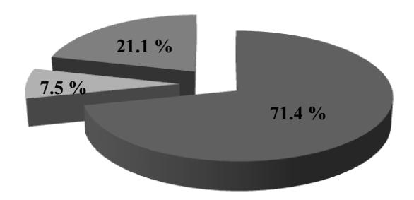
As a consequence of different techniques and different data utilized in the separation process, the results between CST and CSTm differed, as shown in Figure 2. From 4 days of detailed observations performed at different locations throughout 4 major islands of Indonesia, namely Java, Sumatra, Kalimantan and Sulawesi, we obtained 161 different data sets for convective-stratiform separation. As a consequence of differences in method and data used in the separation process, however, there were some discrepancies regarding the separation results between CST and CSTm, as shown in Figure 2. We can see that 71.4% of the data indicate matching separation results between the two methods, whereas 28.6% are marked by mismatching separation results, 7.5% of which indicate occurrences where CST identified a cloud as convective but CSTm identified it as stratiform, 21.1% of which indicate occurrences where CST identified a cloud as stratiform but CSTm identified it as convective.
It is important to note that the separation results are crucial in both CST and CSTm, as they significantly influence the quality of the estimation results.
Discrepancies between the separation results of the two methods suggest differing abilities to estimate rainfall values.
- CST identified separation results as convective when CSTm identified them as stratiform;
- CST identified separation results as stratiform when CSTm identified them as convective;
- CST and CSTm have matching separation results.
Figure 2 Comparison between convective-stratiform separation results of CST and CSTm at 161 different observation points throughout the four major islands of Indonesia.
Even though PMW data are already recognized for their hydrometeor interaction [8, 9,13,18], there has been no strong evidence as to whether they can contribute to applicational advantages. This study, however, hopes to provide the first step for evaluating the benefit of using PMW data in the convective-stratiform separation process.
4.2 Rainfall Estimation
After having performed the separation process, we subsequently proceeded to the estimation of rainfall. Rainfall estimation was performed by using separation results as previously obtained. In this study, the duration of the estimation process as used in both CST and CSTm was 1 hour. Rainfall estimation results and their comparisons against real observation data in different periods and locations are shown in Figures 3, 4, 5 and 6.
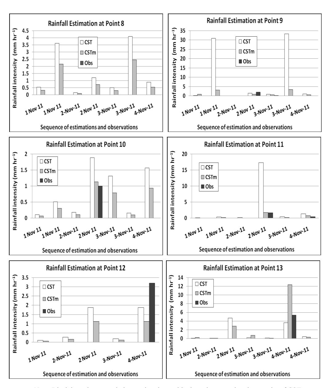
It can be seen that CST and CSTm led to different estimation values, where those of CST were generally higher than those of CSTm, as shown especially in Figures 3, 4 and 5. Real observation values, meanwhile, were generally lower than those of both CST and CSTm. It should be noted that these estimation results could not provide us with an objective conclusion regarding the quality of estimation of either method. For this a verification method was required.
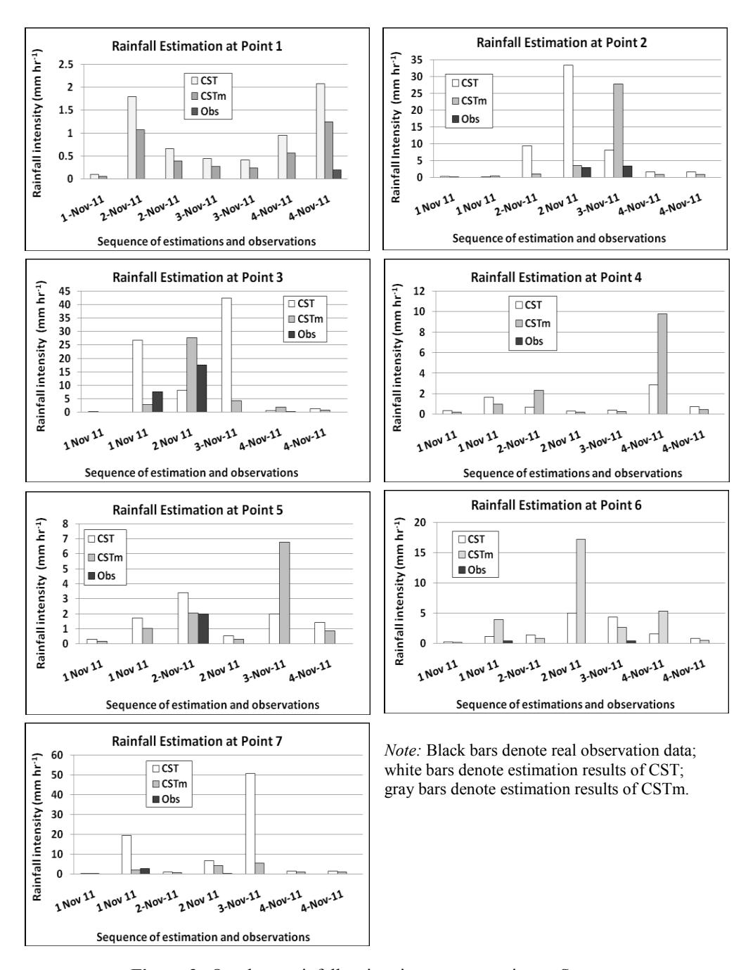
Figure 3 One-hour rainfall estimation at every point on Sumatra.
Note: Black bars denote real observation data; white bars denote estimation results of CST; gray bars denote estimation results of CSTm.
Figure 4 One-hour rainfall estimation at every point on Java.
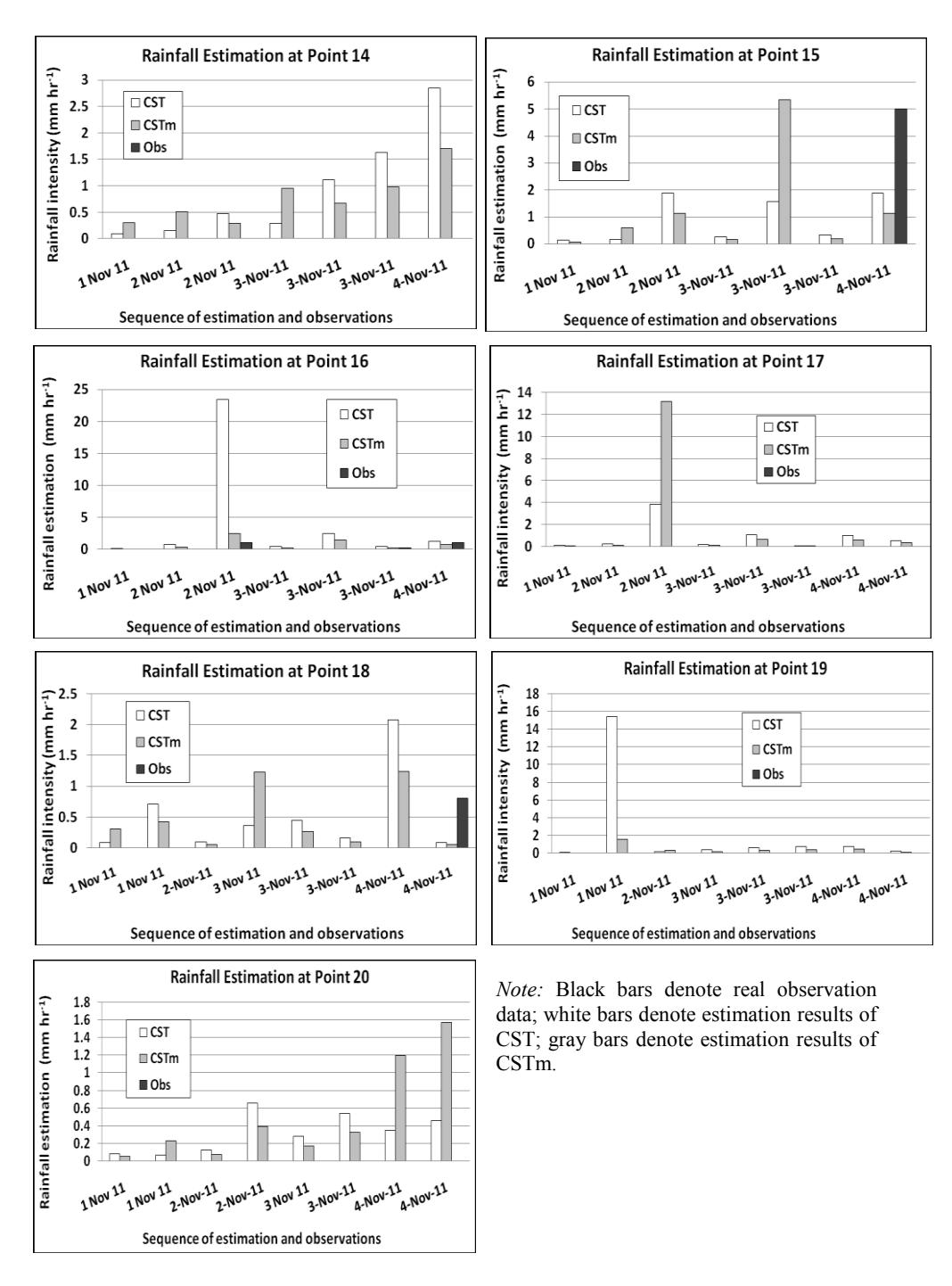
Figure 5 One-hour rainfall estimation at every point in Kalimantan
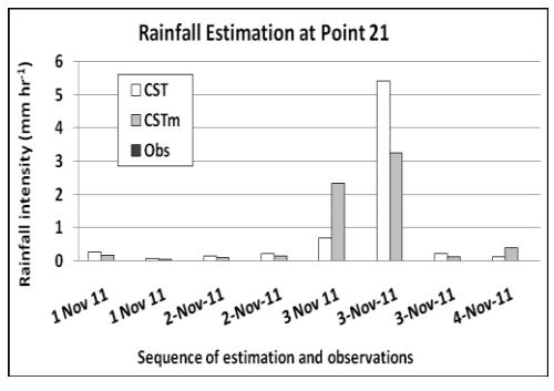
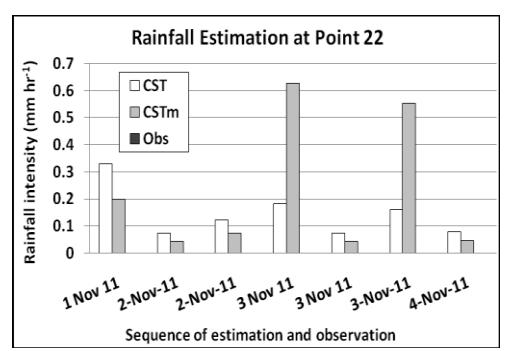
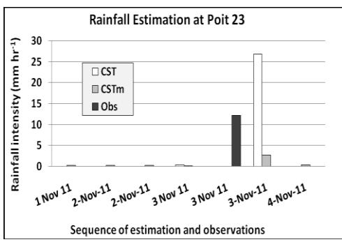
Note: Black bars denote real observation data; white bars denote estimation results of CST; gray bars denote estimation results of CSTm.
Figure 6 One-hour rainfall estimation at every point in Sulawesi.
4.3 Verification Results
In order to verify the estimation results of CST and CSTm as previously obtained, a multi-category contingency table method was applied. This method helped to determine the degree of estimation accuracy of both CST and CSTm, be it on a per location basis or for all locations taken together. We used 4 rainfall intensity categories in the tables, namely no rain, light rain, moderate rain, and heavy to very heavy rain, as shown in Table 3.
4.3.1 Eye Verification (Comparison)
Figure 7 shows a comparison between the degrees of accuracy of both CST and CSTm at each point of observation. These results were obtained by virtue of a multi-category contingency table that was plotted on a per location basis, from point 1 to 23. From this comparison it can be noted that the degree of accuracy of CSTm was mainly better than that of CST, especially for points 1 to 18. In general, the accuracy values of CSTm exceed 0.5, whereas a few of those of CST are below 0.5 (where 1.0 denotes perfect accuracy). From points 19 to 23, however, the degree of accuracy of CST can be seen to be slightly better than that of CSTm. Even so, the accuracy values of both methods generally exceed 0.5.
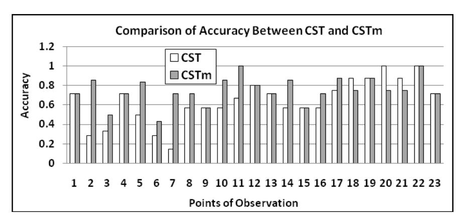
Figure 7 Comparison of accuracy of rainfall estimationat each point of observation.
A recapitulation of the comparison of the accuracy degree of both methods is shown in Table 4: 39.1% suggests a similar degree of accuracy between the two methods; 47.8% suggests CSTm to have better accuracy than CST, while the remainder 13.1% suggests a higher degree of accuracy of CST than that of CSTm.
Table 4 Comparison of accuracy between CSTm and CST.
| Condition | Percentage (%) |
|---|---|
| The CSTm is same with CST | 39.1 % |
| The CSTm is better than CST | 47.8 % |
| The CST is better than CSTm | 13.1 % |
From these verification results, it can be noted that although CSTm is generally a better estimator than CST, this does not always guarantee better results. We are of the opinion that such a limitation is caused by the following factors: i) the PMW data obtained were not the result of direct measurementsof the hydrometeor condition; ii) the spacial resolution of the PMW data obtained was not always consistent, i.e. varying;and iii) there were instances of unavailable observational data as provided by the satellites, most likely due to errors. These factors led to a lower degree of accuracy of CSTm estimation than the authors had hoped to see. However, it is interesting to note that the use of PMW data can be said to have improved both the convective-stratiform separation process and the rainfall estimation process, as supported by the verification results at each observation point.
4.3.2 Categorical Verification
To verify the estimation results for all the observational points taken together, the degree of accuracy of each method was calculated by means of a multicategory contingency table, as shown in Tables 5 and 6.
Table 5 Contingency table of CST for 1-hour estimation and 1-hour rainfall category (accuracy = 0.65).
| Estimation | ||||||
|---|---|---|---|---|---|---|
| 1 | 2 | 3 | 4 | Total | ||
| 1 | 101 | 37 | 7 | 6 | 151 | |
| 2 | 0 | 3 | 1 | 3 | 7 | |
| Observation | 3 | 0 | 0 | 0 | 1 | 1 |
| 4 | 1 | 0 | 1 | 0 | 2 | |
| Total | 102 | 40 | 9 | 10 | 161 | |
Table 6 Contingency table of CSTm for 1-hour estimation and 1-hour rainfall category (accuracy = 0.75).
| Estimation | Total | |||||
|---|---|---|---|---|---|---|
| 1 | 2 | 3 | 4 | |||
| Observation | 1 | 114 | 28 | 6 | 3 | 151 |
| 2 | 1 | 5 | 0 | 1 | 7 | |
| 3 | 0 | 1 | 0 | 0 | 1 | |
| 4 | 1 | 0 | 0 | 1 | 2 | |
| Total | 116 | 34 | 6 | 5 | 161 | |
Where the previous verification (comparison) could only provide a qualitative evaluation by considering each of the observation points, the categorical verification considers all the observation points simultaneously, giving rise to a more quantitative evaluation, as described by Eq. (8). Subsequently, Table 7 shows that the degree of accuracy of CST was 0.65, whereas that of CSTm was 0.75.
Table 7 Accuracy coefficients ofestimation results for CST and CSTm.
| Technique | Accuracy Coefficient |
|---|---|
| CST | 0.65 |
| CSTm | 0.75 |
Up to this point, we can draw a few conclusions from the verification results:
- 1. CSTm is generally better than CST, both qualitatively and quantitatively.
- 2. CSTm is able to improve the quality of estimation of CST, especially for estimations done in Indonesia.
- 3. A convective-stratiform separation process that utilizes the VI method plays a significant role in improving the quality of estimation, as reflected in the accuracy coefficients.
- 4. Using a combination of both PMW and IR data in CSTm's algorithm leads to a better result than merely using IR data (CST).
To further guarantee some degree of consistency in the results, we performed a few more categorical verifications under different circumstances: 1) verifications done for different time periods, namely July 2011 and January 2012; and 2) verifications done as adjusted to an extended rainfall classification.
Tables 8 and 9 show the accuracy coefficients of the rainfall estimations that were done for 3 days in July 2011 (representing the dry season) and 3 days in January 2012 (representing the rainy season).
Table 8 Accuracy coefficients of estimation results for each technique in July 2011.
| Technique | Accuracy Coefficient |
|---|---|
| CST | 0.936 |
| CSTm | 0.974 |
Table 9 Accuracy coefficients of estimation results for each technique in January 2012.
| Technique | Accuracy Coefficient |
|---|---|
| CST | 0.709 |
| CSTm | 0.718 |
As shown in the figures, the accuracy coefficients of CSTm were higher than those of CST, both for July 2011 and January 2012. Consequently, we can conclude that CSTm gives a better quality of estimation, even for different time periods.
Furthermore, we extended the number of rainfall categories from 4 categories to 5 categories, namely no rain (0-1 mm hr-1), light rain (≥1-5 mm hr-1), moderate rain (≥5-10 mm hr-1), heavy rain (≥10-20 mm hr-1), and very heavy rain (≥20 mm hr-1). The accuracy coefficients of both methods as adjusted to the new classification are shown in Table 10.
Table 10 Accuracy coefficients of estimation results with extended classification.
| Accuracy Coefficient | ||||
|---|---|---|---|---|
| Time (Month) | CST | CSTm | ||
| November 2011 | 0.658 | 0.745 | ||
| July 2011 | 0.936 | 0.974 | ||
| January 2012 | 0.689 | 0.709 | ||
From these verification results, it can be seen that the accuracy coefficients of CSTm were always higher than those of CST, even when we extended the number of rainfall categories.
4.3.3 Continuous Verification
To further verify the advantages of using CSTm over CST, we performed a continuous verification involving the calculation of the RMSE values of both methods, as shown in Table 11.
Table 11 The RMSE of the CST and the CSTmat different times
| RMSE | ||||
|---|---|---|---|---|
| Time/Month | CST | CSTm | ||
| November 2011 | 120.320 | 55.890 | ||
| July 2011 | 7.401 | 6.402 | ||
| January 2012 | 49.852 | 30.891 | ||
As can be noted, the RMSE values (margin for errors) of CSTm were always lower than those of CST. We can therefore conclude that CSTm gives better estimations than CST, as there is less room for error in its calculation.
4.3.4 Evaluation of Verification Results
It is easy to see that all methods of verification we have performed supported the claim that CSTm is able to improve the estimation quality of CST, particularly when applied in Indonesia. The improvement is also apparent in the convective-stratiform separation process utilizing the VI method. The change in covered area value as used in the estimation process is also a significant factor that allows the estimation results to be improved. These factors may not seem influential at first, but as we examine the processes as a whole it is apparent that each factor plays an important role in improving the quality of rainfall estimation.
5 Concluding Remarks
We have developed CSTm as a modified method for estimating rainfall that utilizes a combination of PMW and IR data as opposed to only IR data in CST. This method has been proven to be an improvement of CST. It is then desirable to apply the CSTm method as an improved method for providing rainfall estimations. That being said, we do not discourage the practical use of CST. Although its degree of accuracy is lower than that of CSTm, it is still sufficiently high to give reliable rainfall estimations. Furthermore, our analysis suggests that the convective-stratiform separation method plays a significant role in affecting the quality of rainfall estimation. We are of the opinion that a combination of PMW and IR data gives superior results than if one were to use only IR data in the separation process.
Acknowledgements
The authors wish to thank Kochi University Weather Home for providing the infrared weather satellite data and CIRA's AMSU for providing the passive microwave weather satellite data. We would also like to thank the Indonesian Agency for Meteorology, Climatology and Geophysics for providing the hourly rainfall data of some observation points in Indonesia.