1 Introduction

The problems described here have both arisen out of an industrial context. For such problems the objective is normally clear cut. Typically a process is failing and the objective is understand the issues so that a fix can be achieved. Very often the results are important in the specific context but of limited general interest. However it is sometimes the case that the investigation leads to entirely different outcomes than expected, and, if the outcomes are of fundamental and general interest, that is a real bonus. The problems described here are especially rewarding in this regard, and the mathematics required is elementary. The descriptions will be necessarily brief; complete accounts can be accessed in the referred papers.

2 Light Ray Propagation over the Earth

The original question posed was: "Can we accurately determine the path of a light ray propagating over the ocean?". Evidently this is of importance if one wishes to determine the exact location of a ship on the horizon, and is also of importance for short wave communication systems. Although not explicitly expressed in the question the real challenge is to determine the refractive index

profile; we are really dealing with an inverse problem which we well know can be difficult. In this case the inverse problem is known to be almost impossible to solve numerically. The difficulty can be appreciated by observing the very pretty, but complicated, pattern of rays shown in Figure 1, generated by rays projected into a variable refractive index region of very simple form.

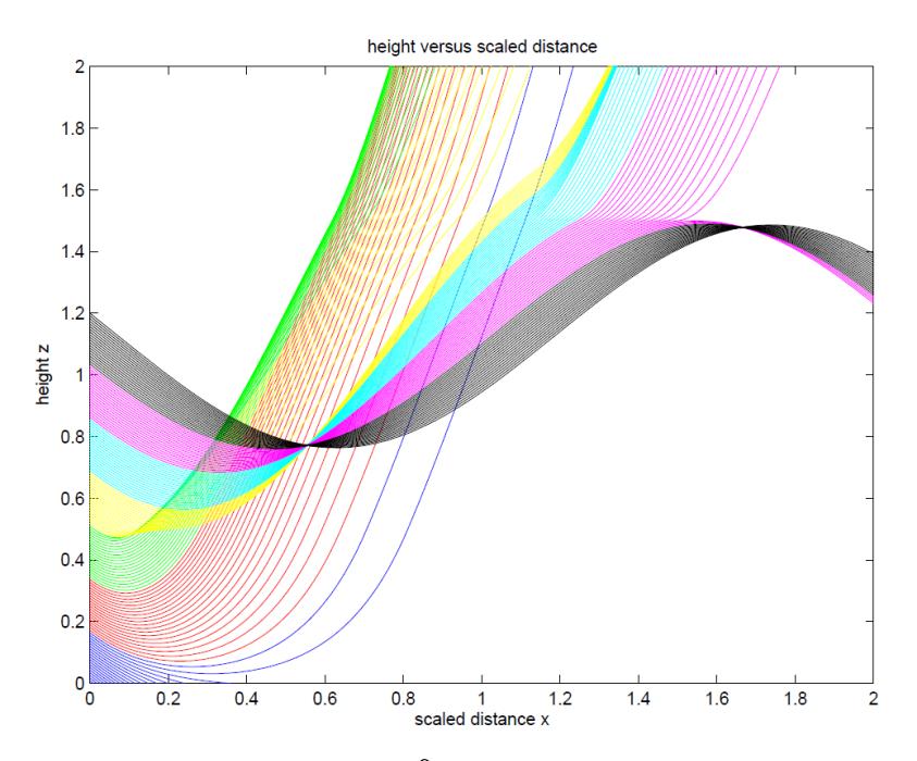
Figure 1 Rays projected from x = 0 at a fixed angle into a variable refractive index medium. The index profile consists of three patched quadratics.

Refractive index variations arise because the speed of ray propagation is (weakly) dependent on the temperature, pressure and humidity of the atmosphere through which the ray is propagating. Significant changes in such climatic conditions occur especially as one moves away from the Earth's surface. The refractive index variations are relatively small \(O(10^{-6})\), so that the deviations of rays from a straight line path are small, however such small variations lead to deflections of the order of 10-20 meters over propagation distances (20-30 km) of interest, and can even be severe enough to cause spectacular effects such as mirages and looming. Over the distances of interest Earth curvature effects also cannot be ignored. A determination of the viewing horizon is often high on the list of priorities.

Given the smallness of variations in refractive index n it is conventional and convenient to describe such variations in terms of the refractivity n' defined by

\[n = 1 + \delta n'\] where \(\delta = 10^{-6}\) (1)

variations in n' of unit order are to be expected in the atmosphere. We will restrict our attention to situations in which the refractivity varies with distance from the Earth's surface.

In a real sense Willebrord Snell knew the solution to the forward problem back in 1621; Snell's Law (when modified for spherical geometry) says

\[rn(r)\cos\gamma(r) = c\]

along a ray, where r is the radial distance within the atmosphere from the Earth's center, n(r) is the refractive index, \(\gamma(r)\) is the angle of the ray with respect to the local horizontal, and c is a constant for the ray. Using this the complete path can be determined by patching together local solutions numerically, see for example [1,2], or by integrating Snell's Law to give an implicit description \(R(\theta)\) for the ray path. Explicitly if the ray is projected from \(r = R_0\) at \(\theta = 0\) at a launch angle whose tangent is \(\gamma_0\) then

\[\int_{R_0}^{R} \frac{q_0 dR'}{R'^2 \sqrt{(n^2(R') - q_0^2 / R'^2)}} = \pm \theta, \text{ with } q_0 = R_0 (1 + \delta n') \cos \gamma_0, \tag{2}\]

see Figure 2, where the sign has to be chosen so that at \(\theta = 0\), \(\gamma = \gamma_0\). For more details see [3]

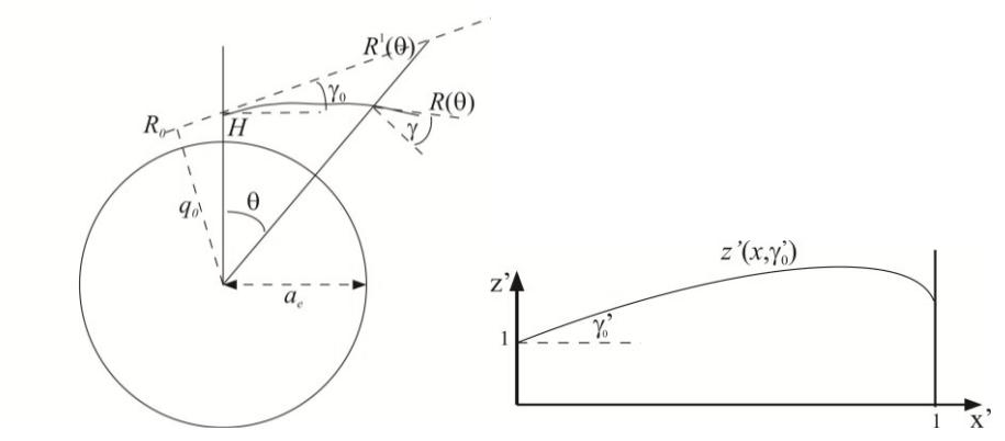
Figure 2 Ray propagation around the Earth: Left: Unscaled geometry. The ray is projected at a height H to a target a distance L around the Earth. Right: The scaled problem.

An explicit evaluation of the integral in (2) is not possible except in the constant refractive index n=1 case, which yields the expected straight line solution \(R^1(\theta)\) given by

\[q_0 / R^1 = \cos(\gamma_0 \pm \theta). \tag{3}\]

Whilst exact, the above ray path description (2) is not suitable for evaluation because of large and small variables and parameters sprinkled throughout the expression. We need to scale the problem, even if only to reduce computational

errors. In fact we'll see that the simple act of scaling leads to a much better result than one would anticipate.

2.1 Scaling

Typically we are interested in waves propagating over distances \(L \approx 10 \mathrm{km}\), at heights \(H = R_0 - a_e \approx 10 \mathrm{m}\), over the Earth, a sphere of radius \(a_e \approx 6 \times 10^3 \mathrm{km}\), within an atmosphere with refractive index variations of the order \(10^{-6}\). With this in mind, we introduce scaled coordinates (x',z'): where x' is the distance from the source location measured around the surface of the Earth and scaled so that x'=1 is the location of the target, and where z' is the height above the surface, scaled so that (0,1) is the location of the source, see Figure 2. To do this we write

\[R = a_e \left( 1 + \left( hl \right) z' \right), \ \theta = l \ x', \ n = 1 + \delta n'(z'), \ \gamma_0 = h \gamma_0'\] \[\tag{4}\] where \[l = \frac{L}{a_e} O(10^{-3}), h = \frac{H}{L} O(10^{-3}), \text{ and } \delta = 10^{-6}\] (5)

After changing to scaled variables, and expanding out in terms of the small parameters \((h, l, \delta)\), the ray path Eq. (2) reduces to

\[x' = \int_{1}^{z'} \frac{1}{\gamma'(n'(u'))} du' + \mathcal{O}(\delta, hl) \text{ where}\] (6)

\[\gamma' = \pm \sqrt{\left[2\eta(n'(z') - n'(1)) + 2\kappa(z' - 1) + (\gamma_0')^2\right]}\] (7)

can be interpreted to be the tangent of the angle the ray path makes with the horizontal at any location z'(x'). Here

\[\eta = \frac{\delta L^2}{H^2}, \ \kappa = \frac{L^2}{a_e H},\tag{8}\] are the dimensionless groups of the problem, a refractivity variation parameter \(\eta\), and an Earth's curvature parameter \(\kappa\); \(\kappa=0\) corresponds to a flat Earth approximation. This may appear to be a purely superficial rearrangement of the earlier description, however from a numerical point of view the improvement is substantial. Both parameters \(\eta\) and \(\kappa\) in the above integral are of unit order and the integral is to be evaluated over a distance of unit order, so that an accurate numerical evaluation is possible using standard packages. If in addition the order \(\delta\), hl terms are neglected (with relative error \(10^{-6}\)) a totally unexpected an extremely important simplification results; the integral in the path description can be evaluated exactly for (up to) quadratic refractive index profiles. In fact exact solutions for the ray path can also be obtained for up to quartic refractive index profiles using the above path description (6), but for reasons that will become evident such evaluations are not useful.

Explicitly if the profile is given by

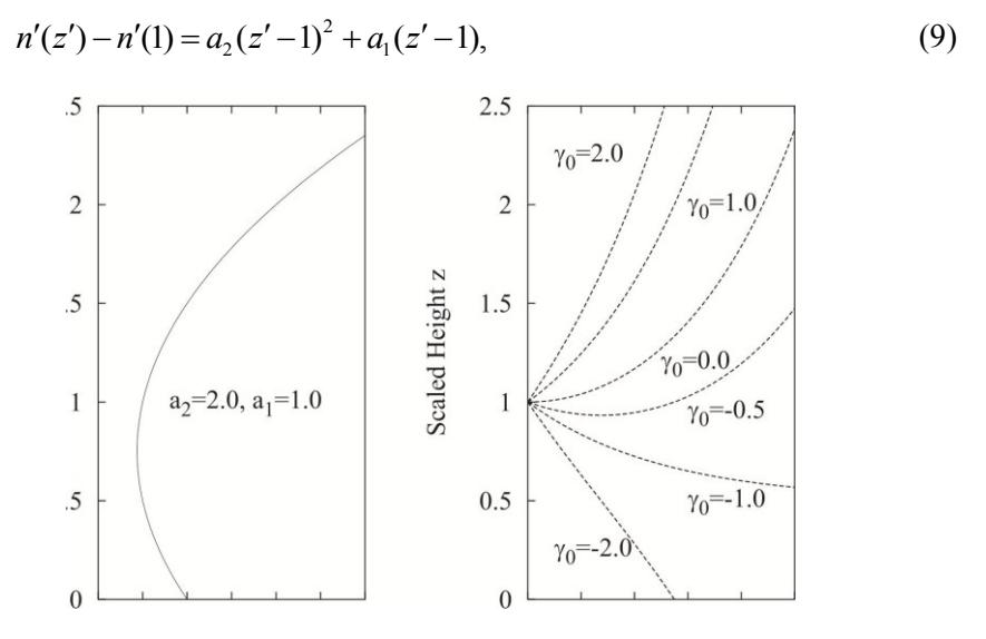
Figure 3 Quadratic Index Profile Rays: \(a_2 < 0\) case. Left: displays the index profile \((a_1 = 1.0, a_2 = 2.0)\). In Right rays are launched from the position z' = 1.0 with a range of initial angles \(\gamma_{0'} = -2 \cdots\), \(\eta = 1\)).

then the integral in (6) can be evaluated to give the explicit path description

\[z' - (1 - \zeta) = \left[\frac{\sin(\sqrt{-2\eta a_2} x')}{\sqrt{-2\eta a_2}}\right] \gamma_{0'} + \zeta \cos\sqrt{-2\eta a_2} x',\tag{10}\] and

\[z' - (1 - \zeta) = \left[\frac{\sinh(\sqrt{-2\eta a_2} x')}{\sqrt{-2\eta a_2}}\right] \gamma_{0'} + \zeta \cos\sqrt{-2\eta a_2} x', \tag{11}\]

In the linear limit \(a_2 = 0\) the familiar parabolic profile

\[z'-1 = \frac{1}{2}[(\kappa + \eta a_1)x'^2 + 2\gamma_0 x'], \tag{12}\] is recovered.

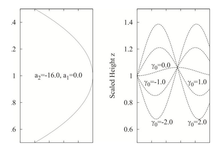
Figure 4 Quadratic Index Profile Rays: \(a_2 < 0\) case. Left: displays the index profile \((a_1 = 0.0, a_2 = -16.0)\). In Right: rays are launched from the position z' = 1.0 with a range of initial angles \(\gamma_{0'} = -1 \cdots\), \(\eta = 1\)).

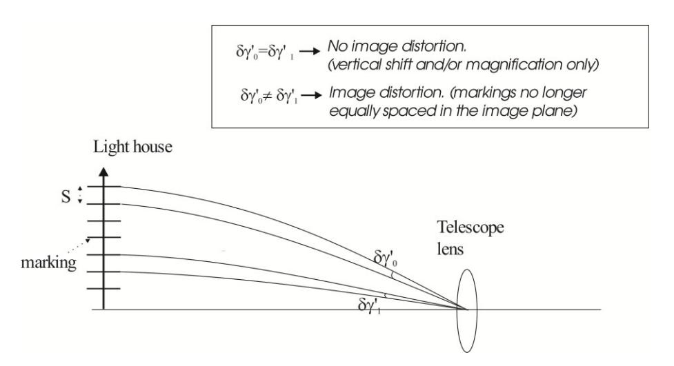
Figure 5 Optical distortion: The figure shows the light ray paths passing through a telescopic lens from equally spaced markings on a lighthouse.

2.2 General Profiles

Evidently the above result enables one to exactly¹ determine image points which is a significant advantage for image inversion, however, what is not so evident but of overriding importance, is that the image generated by rays propagating through a quadratic index profile is undistorted. Now we all know that images are 'true' in a constant refractive index situation (where the rays are straight lines), and many would be aware of the somewhat surprising result that

\(^{^{1}}\) within \(O(10^{-6})\)

images are also 'true' in the linear refractive index profile flat Earth situation (where rays are parabolic). Remarkably, however, this is also the case for quadratic refractive index situations over a spherical Earth! Observing the converging and diverging behavior of propagating rays, see Figures 3, 4, this would seem to be impossible. To understand this result consider rays passing from a target (a lighthouse with equally space markings say) through an observation system (a telescopic lens or the eye) to be viewed in the focal plane of the lens (a photographic plate or the retina), see Figure 5. Now if in fact the angular displacement \(\delta \gamma'_0\) at the lens is the same for all the equally spaced markings (spacing \(\delta z'\) say) from the top to the bottom of the lighthouse then a uniformly magnified or undistorted image will be seen in the focal plane; in fact

\[M = \frac{\partial z'(1, \gamma'_0)}{\partial \gamma'_0}\] measures the local image magnification. More generally we can

identify the offset \({\it O}\) and local magnification \({\it M}\) by writing the path description in the form

\[z'(1, \gamma_0') - z_0'(1, \gamma_0') = O(n', \eta, \kappa) + M(n', \gamma_0, \eta, \kappa)\gamma_{0'}\] where \(z_0'(1,\gamma_0')\) is the image corresponding to \(\gamma_0'\) in the absence of refraction (so n'=n'(1)), and \(z'(n',\gamma_0')\) is the actual image. One might hope that an experimental determination of O and M would enable one to determine the profile n'(z') and thus enable one to invert the image. In general we would expect the magnification M to vary with the entry angle \(\gamma_0'\) so that the image would be distorted, but for the quadratic case using (10,11) we get

\[M(a_2) = \frac{\sin(\sqrt{-2\eta a_2})}{\sqrt{-2\eta a_2}}, O(a_1, a_2) = \frac{\eta a_1 + \kappa}{2\eta a_2} \Big[\cos(\sqrt{-2\eta a_2}) - 1\Big] - \frac{\kappa}{2},\] in the \(a_2 < 0\) case, with similar result in the \(a_2 < 0\) case. Thus the magnification is uniform in the quadratic index profile case. Note also that in this case a single observation of the offset and magnification is sufficient to determine the coefficients \(a_1\), \(a_2\) associated with the index profile, see (9), thus enabling one to simply invert any image received through a quadratic index profile. For higher order profiles distortion occurs.

For more complex profiles than quadratic the received image will be distorted. In such cases, given the above results, it makes sense to use patched quadratics. The ray path through any finite number of quadratic zones can be exactly determined by simply matching the location and slope across the quadratic zones, and thus complete (and effectively exact) images can be generated for any patched quadratic profile. A simple program that does just this has been written and the results are displayed in Figure 6. Of course there is no real need to determine the ray paths; required images can be generated directly using the offset and magnification results above. Note that although pattern of rays is complex it is a relatively simple matter to determine the refractive index

coefficients for each of the layers by measuring the offset and magnification. To determine the thicknesses of the zones one needs to determine/observe the critical rays separating distortionless zones.

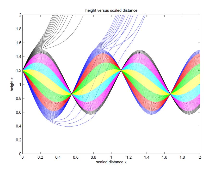
Figure 6 Propagation through three quadratic index layers.

Whilst the evaluations are greatly simplified by the exact evaluation of the path defining integral the most interesting and unexpected aspect of the result is that even for complex profiles consisting of patched quadratics we basically see undistorted images patched together separated by thin distorted zones. I should also add that even mirages are piecewise undistorted, but that is another story. For further details about this and the above work see [4].

3 Boundary Tracing

This is work done by a former student of mine Michael Anderson as part of his PhD, see [5]. The problem concerns the manufacture of capacitors. Capacitors are made by dip coating opposite ends of small (1 mm by 0.5 mm) rectangular silica slabs in molten metal. The results of a single dipping are shown in Figure 7. Note that the contact line between the slab and the metal dips close to the corners of the slab, a condition referred to as mooning. Such mooning is undesirable; the metal caps can break off and excessively mooned capacitors are discarded. The extent of mooning varies even within a particular run. The question was `how to reduce mooning'; for example by altering the properties of the molten metal, rounding the slab edges, or changing the dipping process. Evidently this is a surface tension problem and the determination of the shape of the equilibrium surface of the liquid close to a corner (with wedge angle

\(\alpha = \frac{3\pi}{2}\) in the capacitor case, see Figure 7 is the primary challenge, and challenge it was, and remains. More especially the contact curve between a liquid and the silica slab is of primary interest.

The problem is easy enough to specify. The surface height rise \(\eta(x, y)\) of the liquid in a vessel is governed by the (scaled) Laplace Young equation

\[\nabla \cdot (\frac{\nabla \eta}{\sqrt{1 + \nabla \eta \cdot \nabla \eta}}) = \eta \tag{13}\] in the projection D of the domain occupied by the liquid, see Figure 8 (wedge case), where the length scale adopted is the capillary number \(\sqrt{\sigma/\rho g}\), where \(\rho,\sigma\) are the density and surface tension of the liquid and g is the gravitational constant (see [6]). The contact condition

\[\left(\frac{\nabla \eta}{\sqrt{1 + \nabla \eta \cdot \nabla \eta}}\right) \cdot \mathbf{n} = -\cos \gamma,\tag{14}\]

needs to be imposed around the boundary, where \(\mathbf{n}\) is the external normal to boundary region, and \(\gamma\) is the contact angle, see Figure 8 (infinite wedge case).

The only known exact solution of the Laplace Young equation is the 1D Cartesian solutions discovered by Young. This solution \(\eta(y)\) where y is the distance from the wall is implicitly given by

\[y = \operatorname{arccosh}(2/\eta_w) - \operatorname{arccosh}(2/h) + [\sqrt{4 - h^2} - \sqrt{4 - \eta_w^2}],\] (15)

where \[h = \sqrt{2(1 - \sin \gamma)}\] (see [6]). (16)

is the height rise at the wall, see Figure 9. The height rise in a 1D channel between parallel walls can also be determined using the 1D solution, see [6].

Figure 7 Left: A dip coated slab. Note the contact line between the metal and the slab dips near the corner. Right: The height rise of liquid in a vessel near a corner.

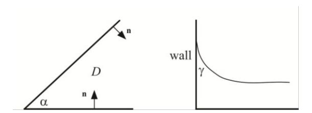
Figure 8 The Laplace Young problem.

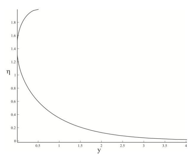
Figure 9 Young's L-Y equation solution.

Obtaining (even) approximate solutions to the Laplace Young equation in other geometries presents real difficulties. Corners in particular present real problems as far as the equation is concerned. It is known that the height rise of a liquid in a wedge is infinite in the corner if the wedge angle , see Figures (7, 8), is less than a critical angle given by ^c / 2 , and is finite and locally planar in a medium wedge angle range ^c . What happens if the wedge angle is larger than , as in the capacitor problem? No one knows complete answers; height discontinuities can even occur. These results are real in the sense that indeed water will defy gravity and climb out of a container with a sharp interior corner. It is known experimentally that if the wedge is rounded sufficiently the water will stay within the container so one might hope to make progress in this case. Michael was set the task of determining the required rounding; he was a very good student! However first he was asked to examine the much simpler but related problem of determining the effect of corner rounding on the solution to Helmholtz equation in the corner plane x y 0, 0 (corresponding to a wedge

angle of 2 ) with a contact condition imposed. Explicitly this involves solving

\[\nabla^2 u = u \text{ in } x > 0, y > 0\] with \[\nabla u \cdot \mathbf{n} = -1\] around \(C\), (17)

see Figure 10.

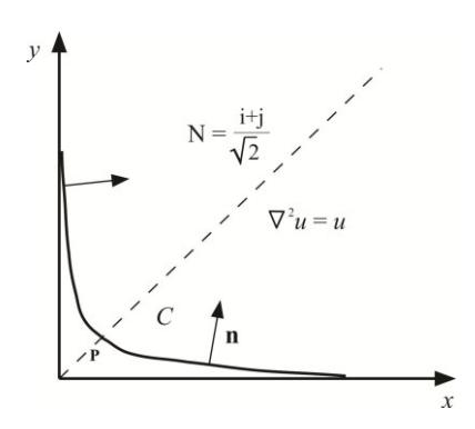
Figure 10 The Helmholtz problem in a rounded quarter plane. The curve C rounds off the corner.

The Helmholtz equation is the small amplitude approximation to the Laplace Young Equation; thus the connection, and of course linearity and the choice of wedge angle simplifies matters greatly. In fact in the absence of rounding the solution is simply given by

\[u^* = e^{-x} + e^{-y}. (18)\]

One might expect a simple perturbation procedure to determine the effect of rounding; it didn't. Even numerical attempts failed! Then something totally unexpected happened that changed everything, and also explained the difficulties. We noticed that the solution \(u^*\) not only solved the contact problem in the quarter plane, but also was the exact solution in a specific rounded domain. To see that there has to be such a domain note that the directional

derivative of \(u^*\) along a line from the origin O at an angle of \(\frac{\pi}{4}\) (so

\(\mathbf{N} = (\mathbf{i} + \mathbf{j})/\sqrt{2}\)) varies from the value \(-\sqrt{2}\) (which is of course less than -1) when (x,y) = (0,0), to zero as the distance from the origin tends to infinity. The implication is that there must be a location P along this line at which \(\nabla u^*(P) \cdot \mathbf{N} = -1\); in fact P is \((\ln(2)/2, \ln(2)/2)\). This point can be used as a starting point for the determination of a complete curve along which the contact condition is satisfied; thus the rounded solution domain can be identified. One would expect the two ends of the resulting curve to asymptote to the two axes. Explicitly if \(\zeta(x,y) = 0\) represents a curve C along which the contact condition (17) is satisfied, then the boundary condition requirement

\[(\nabla \zeta / |\nabla \zeta|) \cdot \nabla u^* = -1\]

determines the slope of the curve C, and this can be used to extend the curve away from the point P. Explicitly if y(x) describes C then the ordinary differential equation

\[\frac{-y'u_x^* + u_y^*}{\sqrt{1 + y'^2}} = -1, \text{ with } y(\frac{\ln(2)}{2}) = \frac{\ln(2)}{2}\]

determines C, with \(u^*(x,y)\) as in (18). Of course one needs to check to see if C asymptotes correctly, but in essence the problem is solved. This is not the only possible curve that can be generated using \(u^*\), although all other such curves have corners. Furthermore there are many other rounding that can be generated for our problem that can be obtained by superposing on \(u^*\) other solutions to the Helmholtz equation with homogeneous Neumann conditions in the quarter plane. For example any of the solutions

\[u^{**} = e^{-x} + e^{-y} + \sum_{n=0}^{\infty} A_n K_n(r) \cos(\beta_n \theta)\], with \(r = \sqrt{x^2 + y^2}\) and \(\beta_n = 2n\pi\), where \(A_n\) is arbitrary could be used. Here \(K_n(r)\cos(\beta_n\theta)\) are radially symmetric source solutions of Helmholtz equation. In this way it is possible to accurately (perhaps even exactly) match a prescribed corner rounding curve C, and thus determine the associated solution.

The above is moderately interesting in its own right but more importantly what we have here is a new procedure for producing exact solution to boundary problems; an entirely unexpected outcome! For obvious reasons we have called this procedure boundary tracing. Note especially that the procedure does not depend on linearity for its application. Given any known specific exact solution of a partial differential equation one can use the above procedure to generate a large number of associated domains with boundary conditions that share the same exact solution. Of course unless the domains generated in this way are practically interesting the technique is little more than a curiosity. However a large number of previously unknown and interesting solutions have already been obtained.

Perhaps most notably he has obtained explicit exact solutions for traced boundaries corresponding to the two known exact solutions of the Laplace Young equation described earlier, see (15). The traced boundary corresponding to the plane wall solution is given by the parametric description

\[x(\eta) = C_1 \pm \frac{\sqrt{2}\cos\gamma}{\sqrt{1-\sin\gamma}} \left[ F\left(\sin^{-1}\left(\left(\frac{2+2\sin\gamma-\eta^2}{4\sin\gamma}\right)\right)^{1/2}\right) \left| \frac{-2\sin\gamma}{1-\sin\gamma} \right) - \frac{1}{1+\sin\gamma} \Pi\left(\frac{2\sin\gamma}{1-\sin\gamma}; \sin^{-1}\left(\left(\frac{2+2\sin\gamma-\eta^2}{4\sin\gamma}\right)\right)^{1/2}\right) \left| \frac{-2\sin\gamma}{1-\sin\gamma} \right] \right]\] \[y(\eta) = \cosh^{-1}\left(\frac{2}{\eta}\right) - \left(\frac{4-\eta^2}{\eta}\right)^{1/2} - \cosh^{-1}\left(\sqrt{2}\right) + \sqrt{2};\] where \(F,\Pi\) are elliptic integrals; a very complex but nevertheless usefully exact result. Examples of these traced solutions are displayed in Figure 11.

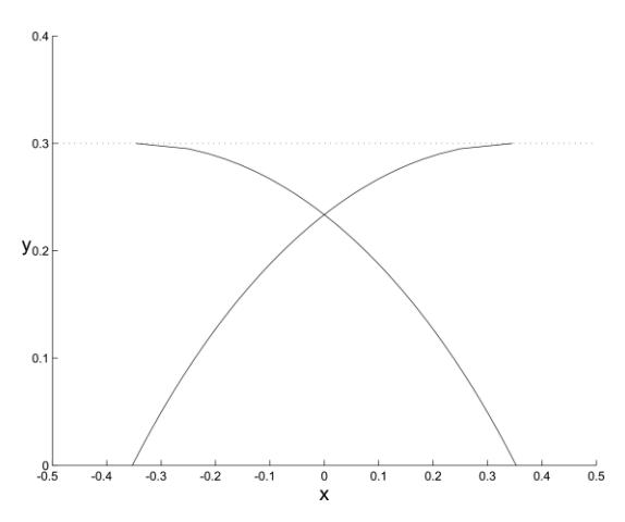
Figure 11 Traced solutions corresponding to Young's solution of the Laplace Young equation.

Figure 12 A variety of boundaries constructed using Young's half plane solution corresponding to the dotted boundary.

Note that solutions are reflected images and that the solutions are invariant under translation in the x direction ( C1 is arbitrary). Solutions associated with the same plane boundary can be patched together to construct a very large class of new domains all of which share Young's 1D solution. Some of these domains are displayed in Figure 12. We believe these results are not only theoretically interesting (greatly increasing the number of know exact results and also providing exact results for corner solutions) but are of major practical importance. One of the major issues that has plagued experimental has been the determination of the effective contact condition for rough surfaces. It has been assumed that rough surfaces behave like plane surfaces but no description for the effect of roughness on the contact angle has been obtained. At least for the very broad range of rough boundaries described above the behavior is exactly the same as that of a plane surface, and the required contact condition is explicitly quantified in the results obtained.

Domains associated with the exact channel solution can also be simply generated using tracing. Of course it is not necessary to have exact solutions to apply the method. For all practical purposes the radially symmetric solution of Laplace Young equation is `known'² . Using this result one can generate

obtainable by integrating the associated ordinary differential equation

interesting circle like and ring like domains; thus one can determine the solution corresponding to rough capillary tubes and rough annular tubes for either the Laplace Young or Helmholtz equation, see Figures 13, 14 and 15 (for Helmholtz equation). Additionally traced boundaries corresponding to the constant mean curvature equation and Poisson's equation have been obtained, see Figure 16. Many of these results have been published in a series of articles and also a preliminary theoretical analysis has been undertaken, see [7,8,9]. However much remains to be done, and it is hoped that this technique will provide a new way of handling nonlinear partial differential equation problems especially.

4 Summary

The two situations examined have produced entirely unexpected outcomes. In the light propagation problem fundamental results concerning the propagation of light rays in the atmosphere were obtained: who would expect the image received in a quadratic refractive index profile to be undistorted and why hasn't this been discovered earlier? In the second situation an entirely new procedure for producing exact solutions to partial differential equations arose out of an industrial surface tension context.

Figure 13 Wedge solutions for Helmholtz equation.

Figure 14 Left: A rough surface solution for Helmholtz equation. Right: Boundary tracing scheme. Grey lines are the individual curves used to generate the boundary.

Figure 15 Boundaries and solutions generated by cylindrical solutions (Helmholtz equation).

Figure 16 Traced boundaries corresponding to Poisson's equation \((\nabla^2 \eta = 1, \text{ with } \nabla \eta \cdot \mathbf{n} = 1)\) using the solutions \(\eta = y^2/2\) (left) and \(\eta = \sin \rho x \sin \rho y\) (right).