
1 Introduction
Mathematical modeling is the process of solving a real-world problem by building mathematical equations based on the phenomena occurring in the problem and then finding their solutions. Ever since ancient Roman times many problems have been solved using mathematical equations. Today, problems in almost all aspects of life, such as industrial manufacturing, economics, politics, social issues and others, can be modeled using mathematics. The result can be a simple model that neglects several factors, or a complex model that requires a higher level of mathematics.
For running the economy, people traditionally use the difference in value of money due to changes in time, so that a borrowing interest rate is applied to loans. However, Islamic law, the Shariah, prohibits riba (interest). Riba in lending money is prohibited in the Islamic economical system (see QS.Ar-Rum: 39 etc. [1]) because it frequently leads to exploitation through unjust and unfair dealings. It is also prohibited by other religions, such as the Jewish and the Christian religion (see Exodus 22:25, Deuteronomy 23:19, Luke 19:22-23, [2]).
In micro-credit lending, the intention to help impoverished people fails frequently due to the occurrence of losses as a result of their economic activity, which can lead to a huge accumulated interest (riba). To circumvent this practice – which eventually becomes an exploitation of impoverished people – the Shariah provides a better concept than taking a definitive interest as a reward when someone offers his/her idle money for borrowing by other people who need cash for making an investment. One thing should be remembered: the money borrowed is strictly for economic activities and not for consumable goods. A profit-loss sharing (PLS) concept gives a reward to the lender with an inconstant base, depending on how much profit or loss the borrower has gained from his/her economic activity. This concept, again, is excellent in theory but seems imperfect in practice. Because the privilege to alter obligation to pay the debt for a particular condition is available, a criminal person can always claim a loss in spite of the actual situation. Indeed, this person practices gharar, which is also prohibited by the Shariah [3,4]. The pursuit of a profit-loss sharing method needs thorough procedures and systems. In sequence, the investor and the trader are prepared well to get involved in this Islamic economic activity. It should be emphasized here that we clearly distinguish between investment and charity money-lending. If the initial intention is charity without the need to pay back, this model cannot be implemented. An investment is classified as musharakah [5-7], also called 'joint equity', when two or more parties collaborate and the investor provides additional funds to the existing trading capital owned by the trader.
Mathematical modeling of PLS schemes has not been studied frequently. In [8], the model is still a simple equation, where financial theories are not considered. The model is improved in [9], but it is still a simple one and not easily applicable. We derived a PLS scheme, first proposed in [10], using financial theories, for example present and future value, and stochastic theories [11], so that the model is dynamic (in time) and easily applicable for micro-credit financing.
In this paper we discuss some problems in the process of making a mathematical model of micro-investments based on a musharakah PLS concept intended to be implemented for low-income traders in a local traditional market. The proposed model of repayment by the trader to the investor will be explained in Section 2. In Section 3, simulation of the generation of profit by the traders and the objective function for optimization of the profit sharing portion in the model are discussed. The determination of the customized values of the parameters used for certain types of traders is explained in Section 4. Notice that in the previous model [10] these parameters were the same for all types of traders.
2 Model of PLS Scheme
In this model, the investor provides a capital, A, and the trader should pay back money daily for a period of T days. The procedure of daily payments is proposed in [12] and, additionally, the traders are deliberately assumed to be women [12,13]. The total amount of payment \(S_t(p)\) at day t consists of the basic installment for repaying the money and a portion of profit sharing, written as follows:
\[S_t(p) = I_t + B_t(p) + C_t, \quad t = 1, 2, ..., T\] (1)
\(I_t\) is the installment at day t for paying the principal. The sharing of profit is determined in variable \(B_t(p)\), which contains profit sharing portion p. \(C_t\) is the payable debt at day t, which will be explained later.
The loss sharing will be reflected in the values of all three variables. If the trader suffers a loss (which will be defined later), she is exempt from paying \(B_t(p)\) and \(I_t\) on that day. However, she still has to pay the basic installment \(I^b\) later, which is accumulated in the debt, \(H_t\). The value of basic installment \(I^b\) is capital A divided by the length of loan period T. Remember that the term debt is used for \(H_t\) due to late payment of the basic installment. There is no penalty for this late payment. Detailed formulation about the basic installment is written below.
\[I^{b} = \frac{A}{T},\] \[I_{t} = \begin{cases} I^{b} & , w_{t} > I^{b}, \\ \frac{w_{t}}{\overline{w}} I^{b}, & 0 \leq w_{t} \leq I^{b}, \\ 0, & , w_{t} \leq 0. \end{cases}\] \[t = 1, 2, ..., T,\]
If the trader's daily profit is larger than basic installment \(I^b\), then the trader needs to pay \(I^b\) in full. If not, which means she has incurred a loss, then either she pays a portion of \(I^b\) or does not pay anything at all. This portion is the ratio
between the daily profit and the average value of the trader's daily profit that is calculated before the scheme begins. When the trader does not pay the basic installment, it will be placed as a debt, accumulated in \(H_t\). At the next occasion when the trader is capable to pay, the debt will be paid as payable debt \(C_t\), t = 2,3,...,T as in Eq. (1). This payable debt can be a full payment of \(H_t\), if she can afford it, or some k sequence of \(C_t\). Below are the formulas for \(H_t\) and \(C_t\).
\[H_{1} = I^{b} - I_{1} , C_{1} = 0\] for \(t = 2, 3, ..., T\) \[C_{t} = \begin{cases} H_{t-1}, & (w_{t} - I^{b} - H_{t-1}) \ge 0 \\ \frac{1}{k} H_{t-1}, & \frac{1}{k} H_{t-1} < w_{t} - I^{b} \le H_{t-1}, \text{ for } k \in \mathbb{N} \\ 0, & (w_{t} - I^{b}) \le \frac{1}{k} H_{t-1}, \text{ for } k \in \mathbb{N} \end{cases}\] \[H_{t} = tI^{b} - \sum_{i=1}^{t} I_{i} - \sum_{j=2}^{t} C_{j}, t = 2, 3, ..., T\]
Now we calculate the profit sharing in case the trader gains a good profit. The calculation of the profit sharing with portion p>0 is formulated in the following equation.
\[B_{t}(p) = \begin{cases} p(w_{t} - I_{t} - C_{t}), & \text{if } (w_{t} - I_{t} - C_{t}) > 0, \\ 0, & \text{if } (w_{t} - I_{t} - C_{t}) \leq 0. \end{cases}\]
Here we determine a good profit by \((w_t - I_t - C_t) > 0\). Having deducted the basic installment \(I_t\) and the payment of debt \(C_t\), the excess profit will be shared with the investor in a portion of p. Finding the optimal value for p is a question of choosing the objective function to be used, which will be answered in Section 4. The trader will have a customized value of p, depending on her trading profit. In the next section, we explain the mechanism of gaining real data from the traders involved in the scheme and generating simulated data on the basis of the real data.
3 Data Simulation and Objective Function Determination
In the micro-credit model [10] we used real data obtained daily from micro-scale traders that had been in trading for quite a long period. Therefore, the averages of their daily profit in the past were available. The traders should be trustworthy in reporting their daily profits. The data were obtained from previous results in [13]. A test showed that they had a log-normal distribution with particular values of mean (drift) and standard deviation (volatility). Based on these real data, we generated data using a simulation in order to have a much larger data set, which is needed for implementation of the optimization method.
For this research, we generated data using geometric Brownian motion. Profit data are defined as follows:
\[w(t) = w(0)e^{\left(\mu - \frac{\sigma^2}{2}\right)t + \sigma\sqrt{t}Z}, Z \sim N(0,1)\] (2)
where \((\mu, \sigma)\) are the mean and standard deviation of the real data.
In the real data some trader's profits are negative, which represents the circumstance in which traders incur a loss in trading. Notice that the data generated in Eq. (2) are always positive. To create the existence of negative profits in the data, we need an additional arrangement after the data are generated. A profit w(t) is negative if a randomly chosen number q > k, where \(q \in [0,1]\) and k is a ratio between the number of positive data and the total number of data.
In Eq. (1), we need to find a portion p such that the model will be optimal, where benefit will be gained by both the investor and the trader. In this optimization problem it is important to define the objective function that satisfies this goal. Define \(r_s(p)\) as the rate of return gained by the investor. This value is obtained from solving the following equation:
\[A = \frac{S_1(p)}{(1+r_c(p))} + \frac{S_2(p)}{(1+r_c(p))^2} + \dots + \frac{S_T(p)}{(1+r_c(p))^T}\](3)
where \(S_t(p)\) is from (1). Also, define \(s_s(p)\) as the portion of the trader's profit that can be taken home daily for the whole period. This value is the following:
\[s_s = \frac{FV(\text{profit-deduction})}{FV(\text{profit})},\tag{4}\] where
\[FV(\text{original-profit}) = w_1 (1 + r_{BI}^d)^{T-1} + w_2 (1 + r_{BI}^d)^{T-2} + \dots + w_T,\] \[FV(\text{deducted-profit}) = (w_1 - S_1(p))(1 + r_{BI}^d)^{T-1} + (w_2 - S_2(p))(1 + r_{BI}^d)^{T-2} + \dots + (w_T - S_T(p)).\]
Here, \(r_{BI}^d\) is the daily rate of interest of the Bank of Indonesia, where
\[r_{BI}^d = \frac{r_{BI}}{252} = 0.028\%\].
Regarding the gain for the investor of this investment, the problem to be solved is
\[\max_{p} r_{s}(p) \tag{5}\]
Constraint: \[r_{BI} < r_s(p) < r_u\]. (6)
The value of \(r_u\) is the rate of return gained by the scheme of an exploiting usurer with the same A and T. A detailed explanation of \(r_u\) can be found in [10].
Regarding the gain for the borrower, the problem to be solved is
\[\max_{p} s_{s}(p) \tag{7}\]
Constraint: \[s_s(p) > s_u\] (8)
Parameter \(s_u\) is the related portion gained by the scheme of an exploiting usurer. Here, the evaluations of functions \(r_s(p)\) and \(s_s(p)\) conflict with each other. If p increases then \(r_s(p)\) will also increase, however, \(s_s(p)\) will decrease.
From this multi-objective optimization problem, we define the objective function as follows:
\[\max_{p} (r_{s}(p) - r_{BI})(s_{s}(p) - s_{u})\] (9)
with constraints, Eq. (6) and (8).
In the next section we make an improvement of the model in [10] by choosing the appropriate values of parameters A and T for particular traders.
4 Determination of Appropriate Values for A and T
The motivation of the need for determining appropriate values of capital A and time period T is the following. At the beginning of research [10], the value of capital A was 1,000,000 IDR (around 10 USD) and T was 52 days for all types of traders. These values are in accordance with the common practice in traditional markets in Indonesia. In fact, however, the profit conditions of the traders vary. There are three types of traders that can be taken from the real
data. Trader type 1 had an average profit of 268,288 IDR, the lognormal data had drift 0.09065 and volatility 2.053498. Trader type 2 had an average profit of 57,884 IDR, the lognormal data had drift -0.003023 and volatility 0.4577. Trader type 3 had an average profit of 48,480 IDR, the lognormal data had drift -0.0050 and volatility 1.315. Some of the real data were not lognormal distributed, so we did not use them. We wanted to know the appropriate values of A and T for which the model gives the optimal result for each type of trader.
In Eq. (3) and (4) there is no explicit relation between \(r_s(p)\) and p, and between \(s_s(p)\) and p. We approximated the relations among them by using a linear regression. The values of \(R^2\) resulted from the linear regression demonstrated strong linearity of \(r_s(p)\) - p and \(s_s(p)\) - p. These linear functions were used for solving Eq. (9). In the next section, we explain the implementation of the model.
5 Implementation
The model has been implemented numerically using MATLAB for \(A = \alpha T \overline{w}\), where \(\overline{w}\) is the average value of w(t), and \(\alpha = \frac{1}{4}, \frac{1}{3}, \frac{2}{3}, \frac{3}{4}, \frac{3}{4}, \frac{3}{2}\). The values for
\(\alpha > \frac{3}{2}\) were not considered, because they make \(s_s(p)\) negative for all types of traders. The values of T were 52, 90 and 180 days. For a couple of A and T values, an implementation of the model will reach the optimal solution at specific values of p, \(r_s(p)\) and \(s_s(p)\). This was then recalculated for a 1000 times and the averages of the obtained values were determined as the optimal solution for given values of A and T. The computation was done for all values of A and T. We show a comparison between them in order to find the appropriate values for A and T for each type of trader.
In Figure 1, where the scale of the vertical axis is adjusted, it is shown that the increase of capital A makes the values of p increase. In contrast, the increase of capital A makes the values of \(s_s(p)\) decrease. On the other hand, the value of \(r_s(p)\) increases at the beginning of the interval, but then decreases at \(\alpha = \frac{2}{3}\) until the end. We can conclude that the optimal value of \(r_s(p)\) will occur when \(\alpha = \frac{2}{3}\) or \(A = \frac{2}{3} \frac{7}{w}\). The behaviours of functions p, \(r_s(p)\) and \(s_s(p)\) are similar for other types of traders.
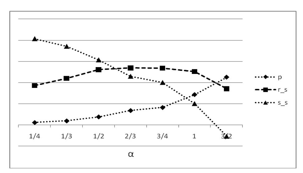
Figure 1 Trader type 1 with T = 52 and various values of A.
In Figures 2-4, the optimal values for ( ) sr p for each type of trader are shown for all values of capital A and period T. The values of ( ) sr p are higher for shorter time periods. The maximum values are the circled ones in the middle of the interval. The maximum values of ( ) sr p for each value of T and its related parameters, p and ( ) s s p , are shown in Table 1. The increase of time period T gives a decrease for both p and ( ) s s p but an increase for ( ) s s p .
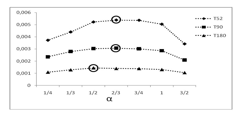
Figure 2 Values of sr for Trader type 1 with various values for A and T.
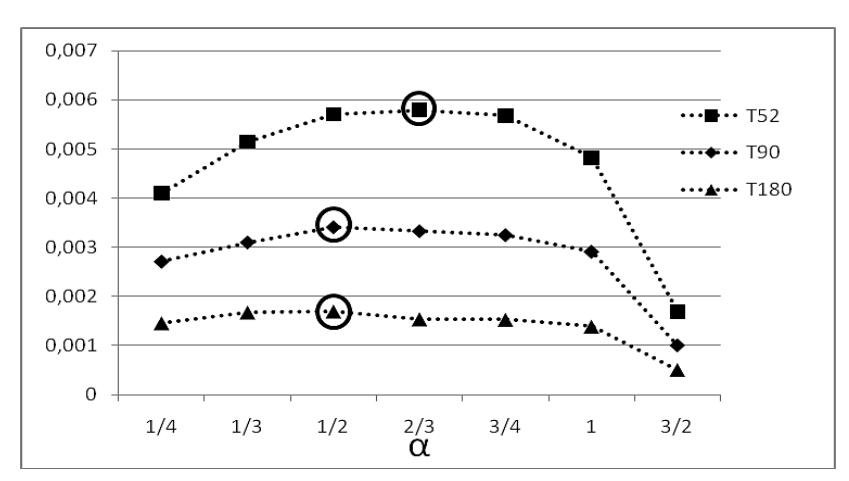
Figure 3 Values of \(r_s\) for Trader type 2 with various values of A and T.
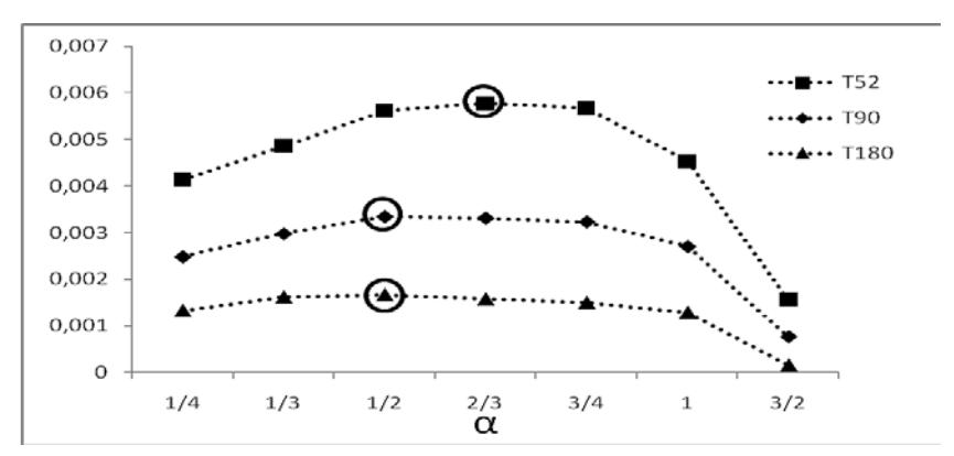
Figure 4 Values of \(r_s\) for Trader type 3 with various values of A and T.
| Table 1 | Values of | parameters for | or different | values of T. |
|---|
| Trader | T=52 | A | T=90 | A | T=180 | A | |
|---|---|---|---|---|---|---|---|
| p | 0.13657 | 0.13188 | 0.08584 | _ | |||
| 1 | \(r_{s}(p)\) | 0.00538 | \(\frac{2}{3}T_{w}^{-}\) | 0.00307 | \(\frac{2}{3}T_{w}^{-}\) | 0.00144 | \(\frac{1}{2}T_{w}^{-}\) |
| \(s_{s}(p)\) | 0.46022 | 3 | 0.47196 | 3 | 0.61418 | 2 | |
| p | 0.19186 | 0.10914 | 0.11263 | ||||
| 2 | \(r_{s}(p)\) | 0.00577 | \(\frac{2}{3}T\overline{w}\) | 0.00335 | \(\frac{1}{2}T_{w}^{-}\) | 0.00167 | \(\frac{1}{2}T\overline{w}\) |
| \(s_s(p)\) | 0.37559 | 3 | 0.53241 | 2 | 0.53488 | ||
| p | 0.18154 | 0.11292 | 0.11478 | ||||
| 3 | \(r_{s}(p)\) | 0.00579 | \(\frac{2}{3}T\overline{w}\) | 0.00341 | \(\frac{1}{2}T_{w}^{-}\) | 0.00170 | \(\frac{1}{2}T_{w}^{-}\) |
| \(s_s(p)\) | 0.38933 | 0.53224 | ۷ | 0.54360 |
6 Discussion and Conclusion
For a particular time period T, the behaviour of value p with respect to an increase of capital A shows that the higher capital A, the larger the portion that needs to be shared with the investor. In this case, even though the values of ( ) s s p decrease, the amount of the deducted-profit in Eq. (4) will increase with respect to changes in A due to the increase of the original profit.
From Table 1, it can clearly be seen that the value of ( ) sr p will decrease along with an increase in the time period, while the value of ( ) s s p will increase. This means the model is beneficial for the trader over longer periods of time.
| Trader | w | T=52 | T=90 | T=180 |
|---|---|---|---|---|
| 1 | 268,288 | 9,300,651 | 16,097,280 | 24,145,920 |
| 2 | 57,884 | 2,006,645 | 2,604,780 | 5,209,560 |
| 3 | 48,480 | 1,680,640 | 2,181,600 | 4,363,200 |
Table 2 The amount of capital A based on optimal values of ( ) sr p .
If we look at the amount of capital A that is optimal for each trader, shown in Table 2, we see that the amount of capital is larger than in the original model [10], where it was 1,000,000 IDR. We can conclude that, using this model, the trader potentially has the capability to manage a larger amount of money according to her profit condition. The larger amount of capital that can be invested is good for the general economy.
We are aware that the obtained conclusions are affected by the simulation method of the data and the choice of the objective function in Eq. (9). In the future, we could use other methods for the data simulation and the determination of the objective function in order to see whether the model still sustains the above conclusions or not.