
1 Introduction
Integer-valued time series models continue to receive an enormous amount of attention. This is not only due to the usefulness of such models for counting processes in many settings, but also due to challenges in the derivation of their statistical properties. One of the important topics in integer-valued time series analysis is the prediction of future realizations. This paper is concerned with prediction for the integer-valued autoregressive process of order one, or INAR(1) process, studied from a frequentist point of view.
Suppose \(\{Y_t\}\) is a discrete-time, stationary, non-negative INAR(1) process satisfying Eq. (1):
\[Y_{t} = \sum_{i=1}^{Y_{t-1}} V_{ti} + \varepsilon_{t}, t \ge 1 \tag{1}\] where the \(V_{ii}\)'s are i.i.d. random variables following a certain (discrete) distribution and the \(\varepsilon_i\)'s are uncorrelated, non-negative, integer-valued random variables. The first term on the right hand side of Eq. (1) may be represented as "\(\theta \circ Y_i\)", see e.g. Al-Osh and Alzaid [1], McKenzie [2], and McKenzie [3], where is the thinning operator. The parameter θ is the probability of 'success' of the random variables Vti , as described in Section 2.
Suppose 1 2 , ,..., YY Yn are observed. Let 1− α denote a future realization of the process, where d is a specified positive integer. Our goal is to obtain an upper prediction limit 1 2 ( , ,..., ) n zY Y Y for Z Y = n d + , such that it has coverage probability, conditional on the last observation, equal to the target nominal value of 1− α , i.e. such that
\[P(Z \le z(Y_1, Y_2, ..., Y_n) | Y_n) = 1 - \alpha\]
Note that because of the Markov property, conditioning on 1 2 ( , ,..., ) YY Yn reduces to conditioning on the last observation Yn for the INAR(1) process.
For the continuous-valued autoregressive (AR) process, the problem of obtaining prediction limits for future realizations and their (conditional) coverage probabilities has been noted by a number of authors, see for example, Barndorff-Nielsen and Cox [4], Vidoni [5], and Kabaila and Syuhada [6]. These authors have constructed prediction intervals or limits with better coverage properties by analytical-based and/or simulation-based approaches.
In this paper, we develop a one-step-ahead upper prediction limit obtained by taking the (1 ) − α -quantile of the conditional probability distribution of a future realization Z . This prediction limit may be a non-integer. Following Vidoni [7], we expand the (1 ) − α -quantile so that
\[z(Y_1, Y_2, ..., Y_n) | Y_n) = \inf\{z \in \Omega_Z : F(z; Y_1, ..., Y_n) \ge 1 - \alpha\}\] where ΩZ is the support and F( )⋅ is the distribution function of Z .
We evaluate the resulting upper prediction limit by calculating its coverage probability, conditional on Y y n n = . It will be shown (in Section 4) through a Monte Carlo simulation that the coverage probability is close to the target nominal. Furthermore, an attempt to modify this prediction limit is carried out, motivated by the work of Kabaila and Syuhada [6]. The aim of this attempt is to find an upper prediction limit with better coverage properties.
The remainder of this paper is organized as follows. In Section 2, the model specification and prediction problem for the Poisson INAR(1) process is described. The construction of prediction limits and their assessment through overage probability is presented in Section 3. We discuss the Monte Carlo simulation in Section 4. Discussion follows in Section 5.
2 Description of the Specification and Prediction Problem for the INAR(1) Process
In the INAR(1) process, assume that the \(V_{ii}\)'s are Bernoulli random variables with probability of 'success' \(\theta\), i.e.
\[P(V_{i} = 1) = 1 - P(V_{i} = 0) = 0\] and also assume that \(\varepsilon_t\) follows a Poisson distribution with parameter \((1-\theta)\lambda\). Then \(Y_t\) has a Poisson distribution with parameter \(\lambda\). We refer to the process in Eq. (1) as a Poisson INAR(1) process.
Let \(\omega = (\theta, \lambda)\). Conditional on \(Y_n = y_n\), the probability mass function of \(Z = Y_{n+d}\) is given by (Freeland [8])
\[p(z \mid y_n; \omega) = P(Z = z \mid Y_n = y_n)\] \[= \sum_{k=0}^{\min(z, y_n)} C_k^{y_n} (\theta^d)^k (1 - \theta^d)^{y_n - k} \frac{1}{(z - k)!} e^{-(1 - \theta^d)\lambda} \{ (1 - \theta^d)\lambda \}^{z - k}\] for z = 0,1,2,... The corresponding moment generating function (mgf) is
\[M(v) = \{\theta^d e^v + (1 - \theta^d)\}^{y_n} e^{-(1 - \theta^d)\lambda} (e^v - 1)\] while the conditional mean and variance are, respectively,
\[E(Z | Y_n = y_n) = \sum_{n=0}^{\infty} zp(z | y_n; \omega) = \theta^d y_n + (1 - \theta^d)\lambda\] and
\[Var(Z | Y_n = y_n) = \sum_{z=0}^{\infty} (z - E(Z | Y_n = y_n))^2 p(z | y_n; \omega)\]
= \(\theta^d (1 - \theta^d) y_n + (1 - \theta^d) \lambda\)
since the \(\varepsilon_n\)'s are independent of \(V_i\), and \(Y_{n-k}\) and the \(\varepsilon_n\) are independent for all \(k \ge 1\).
Let \(z(Y_n; \omega)\) denote the upper prediction limit for Z. It is easy to find \(z(Y_n; \omega)\), for a known \(\omega\), which satisfies the coverage probability \((1-\alpha)\). In practice, however, \(\omega\) is unknown and needs to be estimated from the data. We can then replace \(\omega\) by \(\widehat{\omega}\). The resulting upper prediction limit, \(z(Y_n; \widehat{\omega})\), is called the 'estimative' prediction limit. Our task in the next section is to find this prediction limit and to assess it by calculating its coverage probability.
The estimative prediction limit may be adjusted or modified such that the coverage probability is closer to the target nominal of \((1-\alpha)\). We will call this the 'improved' prediction limit. For a stationary Gaussian AR(1) model, this has been done by authors (for example, Kabaila and He [9] and Vidoni [5]). Whilst some authors have done the adjustment analytically, i.e. through (a) Taylor expansion of the conditional distribution of Z, or (b) predictive density of Z, Kabaila and Syuhada [6] have constructed a simulation-based approach to obtain the improved prediction limit. This method is efficient and can handle complicated models such as Gaussian AR(p) and ARCH(p) processes. Motivated by their work, an attempt of finding an improved prediction limit along with its coverage probability for the case of a Poisson INAR(1) process will be presented.
3 Prediction Limits and Their Coverage Properties
We consider the following d-step-ahead upper \((1-\alpha)\)-estimative prediction limit for \(Z = Y_{n+d}\), Eq. (2):
\[z(Y_n; \hat{\omega}) = (\hat{\theta}^d Y_n + (1 - \hat{\theta}^d) \hat{\lambda}) + q_{1-\alpha} (\hat{\theta}^d (1 - \hat{\theta}^d) Y_n + (1 - \hat{\theta}^d) \hat{\lambda})^{\frac{1}{2}}\] (2)
where \(q_{1-\alpha}\) is the \((1-\alpha)\)-quantile of standard Gaussian distribution. The use of \(q_{1-\alpha}\) is valid due to normal approximation. The conditional coverage probability of [2] is obtained as follows. We observe that Eq. (3):
\[P_{\omega}(Z \leq z(Y_{n}; \widehat{\omega}) | Y_{n} = y_{n})\] \[= P_{\omega}(Z \leq (\widehat{\theta}^{d} Y_{n} + (1 - \widehat{\theta}^{d}) \widehat{\lambda}) + q_{1-\alpha}(\widehat{\theta}^{d} (1 - \widehat{\theta}^{d}) Y_{n} + (1 - \widehat{\theta}^{d}) \widehat{\lambda})^{\frac{1}{2}} | Y_{n} = y_{n}) \quad (3)\] \[= E_{\omega}(F((\widehat{\theta}^{d} Y_{n} + (1 - \widehat{\theta}^{d}) \widehat{\lambda}) + q_{1-\alpha}(\widehat{\theta}^{d} (1 - \widehat{\theta}^{d}) Y_{n} + (1 - \widehat{\theta}^{d}) \widehat{\lambda})^{\frac{1}{2}}) | Y_{n} = y_{n})\]
The conditional expectation Eq. (3) is estimated by simulation. To do this, we use the method of Kabaila [10], which will be described in Section 4. All the computations were carried out with programs written using MATLAB and its Statistics Toolbox.
Now, to obtain a better coverage probability property, i.e. closer to the target value, we adjust the above estimative prediction limit, Eq. (2). The main idea behind this adjustment is to absorb the correction term as the result of estimating Eq. (3). Accordingly, we define
\[c(\omega, y_n) = P_{\omega}(Z \le z(Y_n; \widehat{\omega}) | Y_n = y_n) - (1 - \alpha)\] so that the order \((1-\alpha)\) is the same as the order of the correction term of the coverage probability of the estimative prediction limit, Eq. (3). The improved prediction limit is given by Eq. (4):
\[z^*(Y_n; \widehat{\omega}) = z(Y_n; \widehat{\omega}) + d(\omega, y_n)\] (4)
where \(d(\omega, y_n)\) is such that
\[c(\omega, y_n) + \sum_{i=1}^{d(\omega, y_n)} p(z(Y_n; \widehat{\omega}) | y_n) + i; \omega) \leq 0,\] for \(c(\omega, y_n) < 0\). The coverage probability of [4], conditional on \(Y_n = y_n\), is given by Eq. (5):
\[P_{\omega}(Z \le z^{*}(Y_{n}; \widehat{\omega}) | Y_{n} = y_{n}) = P_{\omega}(Z \le z(Y_{n}; \widehat{\omega}) + d(\omega, y_{n}) | Y_{n} = y_{n})\] \[= E_{\omega}(F_{Z}(z(Y_{n}; \widehat{\omega}) + d(\omega, y_{n})) | Y_{n} = y_{n})\] (5)
and we estimate it by simulation. For \(c(\omega, y_n) > 0\), we find \(d(\omega, y_n)\) such that
\[\sum_{i=1}^{d(\omega, y_n)} p(z(Y_n; \widehat{\omega}) | y_n) + i; \omega) \le c(\omega, y_n).\]
The improved prediction limit is Eq. (6):
\[z^*(Y_n; \widehat{\omega}) = z(Y_n; \widehat{\omega}) - d(\omega, y_n)\] (6)
A detailed description of how the Monte Carlo simulation estimates were carried out will be provided in the next section. It will be shown that there is improvement in the coverage properties of the improved prediction limit, compared to that of the estimative limit.
4 Monte Carlo Simulation
In this section, Monte Carlo simulation estimates are presented to obtain a one-step-ahead upper estimative prediction limit and improved prediction limit (the case of d=1) along with their coverage probability. We begin by obtaining simulated data from a Poisson INAR(1) model, with sample sizes n=50 and n=100, for \(\theta=0.1,0.2,0.5,0.75\) and \(\lambda=2\). We have used the following Yule-Walker estimators
\[\hat{\theta} = \frac{\sum_{t=1}^{n-1} (Y_t - \hat{Y})(Y_{t+1} - \hat{Y})}{\sum_{t=1}^{n} (Y_t - \overline{Y})^2} \text{ and } \hat{\lambda} = \frac{1}{n-1} \sum_{t=2}^{n} (Y_t - \hat{\theta} Y_{t-1})\] to estimate \(\theta\) and \(\lambda\), respectively. The reason for using these estimators is that the method of Kabaila and Syuhada [6] is also applicable for any estimators other than either a maximum likelihood estimator or a conditional maximum likelihood estimator.
Now, to estimate [3] by using the simulation algorithm of Kabaila, we first define \(X = (Y_1, ..., Y_{n-1})\) and \(Y = Y_n\). Thus, the conditional expectation in Eq. (3) is equal to
\[E_{\omega}(h(X,y)|Y=y)\] where
\[h(X, y) = F_Z((\hat{\theta}y_n + (1 - \hat{\theta})\hat{\lambda}) + q_{1-\alpha}(\hat{\theta}(1 - \hat{\theta})y_n + (1 - \hat{\theta})\hat{\lambda})^{\frac{1}{2}})\] and \(y = y_n\). Meanwhile, the probability density function of Y, conditional on X = x, P(Y = y | x), is given by
\[P(Y = y \mid X = x) = \sum_{k=0}^{\min(y,x)} C_k^x \theta^k (1 - \theta)^{x-k} \frac{1}{(y-k)!} e^{-(1-\theta)\lambda} \{ (1-\theta)\lambda \}^{y-k}\] for y = 0,1,... Thus, the estimate of Eq. (3) is
\[\frac{\sum_{r=1}^{M} P(Y = y \mid X^{r} = x^{r}) h(x^{r}, y)}{\sum_{s=1}^{M} P(Y = y \mid X^{s} = x^{s})}\] for M independent simulation runs. It is noted that the standard error of this estimate is calculated by Theorem 4.2 of Kabaila [10].
The performance of the coverage probability of the estimative prediction limit for the Poisson INAR(1) model are provided in Table 1 and Table 2, based on 200 replications. The values close to the target nominal and the standard error were reasonably small, except when \(\theta = 0.5\). The coverage probability, conditional on \(Y_n = 2\), for various \(\lambda\) (\(\theta = 0.1\)) is presented in Figure 1. The number of simulation runs was 200 for a sample size of 100. The coverage probability was far from the target value as \(\lambda\) increased.
To find the improved prediction limit and its coverage probability, we considered the case that \(\theta = 0.2\) and \(\lambda = 2\) with the number of samples is 50. The estimative 0.95 prediction limit \(z(Y_n; \hat{\theta}, \hat{\lambda}) = 5\). The coverage probability, conditional on \(Y_n = 3\), was calculated based on 200 replications. We obtained Eq. (2) is equal to 0.9390(0.0014). The improved prediction limit obtained is 6.
Table 1 Estimated conditional coverage probabilities of the estimative 0.95 prediction limit for Poisson INAR(1) Model (\(\lambda\)=2), conditional on Yn=2,3. Standard errors are in brackets.
| n | θ | \(Y_n = 2\) | \(Y_{n} = 3\) |
|---|---|---|---|
| 50 | 0.1 | 0.9507(0.0018) | 0.9502(0.0016) |
| 0.2 | 0.9347(0.0029) | 0.9390(0.0014) | |
| 0.5 | 0.9063(0.0025) | 0.9285(0.0013) | |
| 0.75 | 0.9445(0.0007) | 0.9517(0.0025) | |
| 100 | 0.1 | 0.9507(0.0014) | 0.9470(0.0012) |
| 0.2 | 0.9412(0.0021) | 0.9356(0.0008) | |
| 0.5 | 0.8918(0.0010) | 0.9293(0.0001) | |
| 0.75 | 0.9483(0.0001) | 0.9556(0.0001) |
Table 2 Estimated conditional coverage probabilities of the estimative 0.90 prediction limit for Poisson INAR(1) Model (\(\lambda\)=2), conditional on \(Y_n\)=2,3. Standard errors are in brackets.
| n | θ | \(Y_n = 2\) | \(Y_{n} = 3\) |
|---|---|---|---|
| 50 | 0.1 | 0.9134(0.0032) | 0.9229(0.0026) |
| 0.2 | 0.8898(0.0030) | 0.9064(0.0033) | |
| 0.5 | 0.8906(0.0017) | 0.8557(0.0059) | |
| 0.75 | 0.8920(0.0081) | 0.8496(0.0082) | |
| 100 | 0.1 | 0.9109(0.0032) | 0.9296(0.0025) |
| 0.2 | 0.8816(0.0027) | 0.9098(0.0030) | |
| 0.5 | 0.8890(0.0000) | 0.8314(0.0057) | |
| 0.75 | 0.9005(0.0074) | 0.8156(0.0060) |
Note that the improved prediction limit may not be found unless it satisfies the following condition
\[\sum_{i}^{\min_{i}} p(z(Y_{n}; \widehat{\omega}) + i; \omega) \leq -c(\omega, y_{n})\] for \(c(\omega, y_n) < 0\). The example can be observed from Table 1, when n = 100, \(\theta = 0.1\) and \(\lambda = 2\), in which the coverage probability, conditional on \(Y_n = 3\), is 0.9470. Here, \(c(\omega, y_n) = -0.003\). The estimative prediction limit is 4.4667,
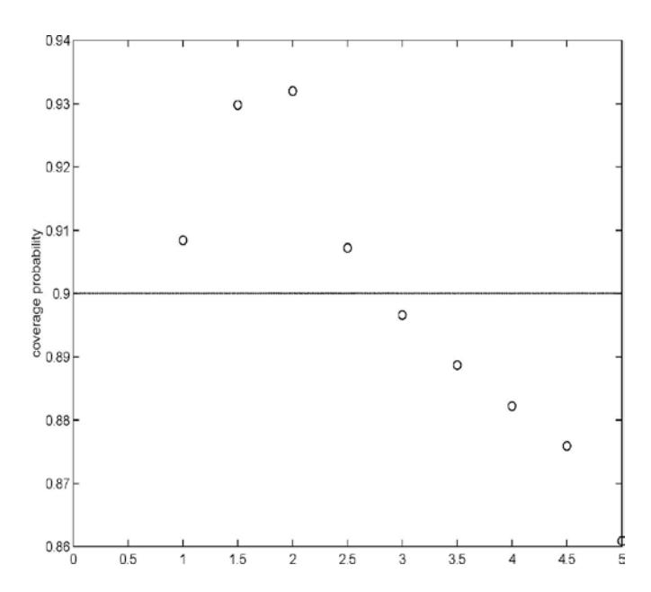
Figure 1 Conditional Coverage Probabilities of the 0.90 Estimative Prediction Limit for various ( 0.1, 2, 100) λ θ= = = Y n n with 200 replications.
which can be rounded to either 4 or 5. We expect the improved prediction limit to be longer than the estimative one. However, either p = 5 or p = 6 has a value greater than 0.003. Thus, we conclude that the improved prediction limit is the estimative one. In other words, our best prediction limit is the estimative prediction limit.
5 Discussion
The use of Kabaila's method [10] to estimate the conditional coverage probability may be avoided if we can have the backward representation of the Poisson INAR(1) process. Note that, for the AR( p ) process, the backward representation is obtained only if we assume normality for the error of the process.
Unlike the continuous-valued autoregressive process, the INAR process may not always give us the improved prediction limit due to its discreteness and expectation to obtain a coherent prediction. The possible improved prediction limit really depends on the value of (, ) n c y ω . As mentioned in Section 4, a similar condition should also be satisfied when (, ) 0 n c y ω > , in which the minimum sum of (( ; ) ; ) n pzY i ω− ω should be greater than or equal to (, ) n c y ω .
Acknowledgements
The first author is grateful to King Saud University. The first and second authors are indebted to the conference organizers of CSOR for their invitation to present this paper and their very warm hospitality. The authors would like to express their thanks to Prof. Ravi Shankar and two anonymous referees for suggestions to improve the presentation of the paper.