
1 0BIntroduction
Lanczos-type algorithms are effective methods to solve systems of linear equations (SLE). One of their attractions is that, in exact arithmetic, they achieve an exact solution in n steps where n is the dimension of the problem [1]. However, they have a weakness linked to their need to estimate the coefficients of the orthogonal polynomials used in the recurrence relationships on which they are based. For instance, when the denominator of any of these coefficients is zero, then the corresponding orthogonal polynomial does not exist; the solution process stops and fails to reach the solution. This is known as the breakdown phenomenon. There are many forms of this, such as hard, soft, curable, incurable [2], true, and ghost breakdowns [1,3]. Here, we are concerned with true or hard breakdown.
Note that the more iterations we do, the more likely breakdown will occur. Since we do not work in exact arithmetic, to get good approximate solutions, a number of iterations exceeding the dimension of the problem is often required. Therefore, breakdown is even more likely to occur. That is why Lanczos-type algorithms suffer from breakdown and that is why approaches to dealing with this problem are continually being developed [4-6].
There are already many strategies to tackle breakdown, such as the look-ahead strategy [7], also called the method of recursive zoom (MRZ), and the lookaround strategy [8,9]. These typically try to get over and/or around the nonexisting orthogonal polynomials. Attempts based on different strategies, such as switching between Lanczos-type algorithms and restarting them, have also been considered [4-6]. These latter approaches have been shown to perform better than MRZ in terms of robustness [5,6].
In this paper, we will focus on restarting from three specific points which are attractive as starting points: the last iterate preceding breakdown, the iterate with the lowest residual norm, and the iterate whose entries are the median values of all entries of the iterates generated so far.
It is reasonable to restart from the point immediately before the breakdown occurred since this leads one to believe that the sequence that has been broken is continued somehow, albeit in a different Krylov space. However, there is no theoretical evidence for this. Indeed, it may be counter-productive since just before breakdown the quality of the iterates deteriorated from the point of view of the residual norm. Our numerical results support this view, as will be seen later.
Restarting from the iterate with minimum residual norm in the sequence of solutions generated so far is also reasonable since we now have a good starting point which is not just a guess. Numerical results included here, also support this idea.
Finally, restarting from an approximate solution whose entries are the median of the entries of all the iterates generated so far also sounds like a reasonable starting point. This is because one might think that the median values of the entries capture the intrinsic qualities of the sequence of solutions found so far. However, it is also clear that it will include information from points that are very bad since they lead to the process of blowing up (breakdown) in terms of their residual values. As one would expect, the results point to this artificially made-up iterate as being in between the other two in terms of quality.
We will also look at the theoretical aspect of restarting. This has been considered previously in [2,10]. Numerical results obtained on problems ranging from 1000 to 70000 dimensions will be provided.
2 Lanczos-type Algorithms for SLE's and the Issue of Breakdown
2.1 Lanczos-type Algorithms: Review
Consider the system of linear equations
\[A\mathbf{x} = \mathbf{b},\tag{1}\] where ∈ and vectors and ∈ . Lanczos-type methods for solving Eq. (1) can be derived by combining the method of Krylov subspace and the method of projections, [11]. It is started by choosing an initial approximate solution 0 and defining the sequence of vectors by two conditions:
\[\mathbf{x}_k - \mathbf{x}_0 \in K_k(A, \mathbf{r}_0), \tag{2}\] and
\[\mathbf{r}_k = \mathbf{b} - A\mathbf{x}_k \perp L_k = K_k(A, \mathbf{y}), \qquad (3)\] where 0 = – 0 is the corresponding residual vector, is an arbitrary nonzero vector, and (, 0) is a Krylov subspace. From Eq. (2) we have:
\[\mathbf{x}_k - \mathbf{x}_0 = -\alpha_1 \mathbf{r}_0 - \alpha_2 A \mathbf{r}_0 - \dots - \alpha_k A^{(k-1)} \mathbf{r}_0. \tag{4}\]
Thus, multiplying both sides by , adding and substracting , we obtain:
\[A(\mathbf{x}_{k} - \mathbf{x}_{0}) = A \left(-\alpha_{1}\mathbf{r}_{0} - \alpha_{2}A\mathbf{r}_{0} - \cdots - \alpha_{k}A^{(k-1)}\right)\mathbf{r}_{0},\] \[A\mathbf{x}_{k} - A\mathbf{x}_{0} = -\alpha_{1}A\mathbf{r}_{0} - \alpha_{2}A^{2}\mathbf{r}_{0} - \cdots - \alpha_{k}A^{k}\mathbf{r}_{0},\] \[\mathbf{b} - \left(A\mathbf{x}_{k} - A\mathbf{x}_{0}\right) = \mathbf{b} + \alpha_{1}A\mathbf{r}_{0} + \alpha_{2}A^{2}\mathbf{r}_{0} + \cdots + \alpha_{k}A^{k}\mathbf{r}_{0},\] \[\mathbf{b} - A\mathbf{x}_{k} = (b - A\mathbf{x}_{0}) + \alpha_{1}A\mathbf{r}_{0} + \alpha_{2}A^{2}\mathbf{r}_{0} + \cdots + \alpha_{k}A^{k}\mathbf{r}_{0},\] \[\mathbf{r}_{k} = \mathbf{r}_{0} + \alpha_{1}A\mathbf{r}_{0} + \alpha_{2}A^{2}\mathbf{r}_{0} + \cdots + \alpha_{k}A^{k}\mathbf{r}_{0}.\] (5)
From the last relation, we can write
\[\mathbf{r}_k = P_k(A)\mathbf{r}_0,\tag{6}\] where () = 1 + 1 + ⋯ + is of degree at most, and satisfies the normality condition (0) = 1.
Following the definition of the family of orthogonal polynomials given in [3], we set \(c_i = \langle \mathbf{y}, A^i \mathbf{r}_0 \rangle\), with c a linear functional on the vector space of polynomials defined by
\[c_i = c(x^i), \quad i = 1, 2, \cdots \tag{7}\]
The condition Eq. (6) can be written as
\[c(t^{i}P_{k}(t)) = 0, i = 0,1,...,k-1,\] (8)
which shows that \(P_k\) is the polynomial of degree k at most, normalized by \(P_k(0) = 1\), belonging to the family of orthogonal polynomials with respect to functional c. Thus, the Lanczos method consists of determining implicitly the polynomial \(P_k\), computing recursively the residual \(\mathbf{r}_k = P_k(A)\mathbf{r}_0\), and finding \(\mathbf{x}_k\) from \(\mathbf{x}_k = \mathbf{b} - A\mathbf{r}_k\) without inverting the matrix A.
Some Lanczos-type algorithms have been discussed by Brezinski and his team, which are expressed in a table containing formulae \(A_i\) and \(B_j\), [12-14]. Basically, the computations of the recurrence relations are based on \(P_k\) and \(P_k^{(1)}\) respectively, with degrees of the polynomials on the right and left hand sides differing by one or two degrees at most. The new formulae which involve the polynomials with a difference in degrees of at most two or three can be seen in [4,15].
2.2 The Breakdown Phenomenon
Breakdown in Lanczos-type algorithms can be caused by either the non-existence of some orthogonal polynomials or because the recurrence relationship used is not appropriate. Following the explanation in [16], consider how breakdown occurs when estimating the coefficients of orthogonal polynomials.
Consider the three term recurrence relationship of the monic polynomial \(P_{k+1}\) as follows:
\[P_{k+1}(t) = (\alpha t + \beta) P_k(t) + \gamma P_{k-1}(t), \tag{9}\] where \(k=0,1,\cdots\). This polynomial satisfies the conditions: (1) \(P_{-1}(t)=0\), (2) \(P_0(t)=1\), and (3) \(c(t^iP_k)=0\), for \(i=0,1,\cdots,k-1\), where c is a linear function. The last condition, which is also known as the orthogonality condition, gives:
\[c(t^{i} P_{-}k + 1) = \alpha c(t^{i} + 1 P_{-}k(t)) + \beta c(t^{i} P_{-}k(t)) + \gamma c(t^{i} P_{-}(k - 1)(t)),\] (10)
For \(i = 0,1,\dots,k\). In particular, for i = k-1 and i = k we get relations
\[0 = \alpha c(t^k P_k(t)) + \gamma c(t^k - 1 \{P_k - 1(t)\})\] (11)
\[0 = \alpha c \left( t^k + 1 P_k(t) \right) + \beta c \left( t^k P_k(t) \right) + \gamma c \left( t^k P_{k-1}(t) \right)\] (12)
respectively. The second condition leads to the equation,
\[1 = \beta + \gamma. \tag{13}\]
As we can see, we now have a system of linear equations in \(\alpha\), \(\beta\), \(\gamma\). Solving for \(\alpha\), \(\beta\), \(\gamma\) gives:
\[\alpha = 1\] \[\gamma = \frac{-c(t^{k}P_{k}(t))}{c(t^{k-1}P_{k-1}(t))},\] \[\beta = \frac{\gamma c(t^{k}P_{k-1}(t)) - c t^{k+1} P_{k}(t)}{c(t^{k}P_{k}(t))}.\] (14)
In order for relation Eq. (9) to be finite, the scalars \(c\left(t^{k-1}P_{k-1}\left(t\right)\right)\) and \(c\left(t^{k}P_{k}\left(t\right)\right)\) must not be zero, or sufficiently close to zero, i.e. small enough to cause an NaN output in the computation. Otherwise, a breakdown occurs.
3 Restarting Lanczos-type Algorithms
Here, we introduce the different implementations of restarting Lanczos-type algorithms from three different points. RLLastIt restarts from the last iterate; RLMinRes restarts from the iterate with the minimum residual norm; RLMedVal restarts from a point made up of the median values of all the entries of previous iterates in a sequence generated by the Lanczos-type algorithm under consideration. Restarting in all cases is of the pre-emptive type as described in [5].
3.1 Restarting Lanczos-type Algorithms from the Last Iterate
Assume that we stop the algorithm after k iterations. Also assume that breakdown does not occur within k iterations. Note that a high k means the algorithm may break down. Consider the iterate \(\mathbf{x}_k\), as the last iterate, with residual norm \(\|\mathbf{r}_k\|\). Initialize the algorithm as follows,
\[\mathbf{x}_0 = \mathbf{x}_k \tag{15}\]
\[\mathbf{y} = \mathbf{b} - A\mathbf{x}_0 \tag{16}\]
RLLastIt is described in Algorithm 1.
Algorithm 1 The RLastIt Algorithm.
- 1. Fix the number of iterations to, say, k, and the tolerance, \(\epsilon\), to 1E-13.
- 2. Run a Lanczos-type algorithm for k iterations and get the approximate solution \(sol_{last} = \mathbf{x}_k\), as well as the residual norm \(norm_{last} = ||\mathbf{r}_k||\).
- 3. while \(norm_{last} \ge \epsilon\) do
- 4. Initialize the algorithm with
\[\mathbf{x} = sol_{last},\]
\(\mathbf{y} = \mathbf{b} - A \mathbf{x}.\)
- 5. Run the Lanczos-type algorithm for k iterations.
- 6. endwhile.
- 7. Take \(sol_{last}\) as the approximate solution.
- 8. Stop.
3.2 Restarting Lanczos-type Algorithms from the Iterate with the Minimum Residual Norm
Because of the potential accumulation of errors, the last iterate after k iterations is not necessarily the one with the smallest residual norm. It is therefore reasonable to consider restarting from the point among the k iterates with the lowest residual norm. Figure 1 illustrates the residual norm behaviour of the iterates after running the Orthodir algorithm [12] when solving problems in 300 dimensions using 150 iterations. This figure describes the situation mentioned earlier that the last iterate is not always the best one. In this case, the iterate with the lowest residual norm is the \(29^{th}\).
To run RLMinRes, we collect all of the iterates generated in k iterations and their residual norms.
\[data_{sol} = \{\mathbf{x}_1, \mathbf{x}_2, \dots, \mathbf{x}_k\},\tag{17}\]
\[data_{resnorm} = \{ \|\mathbf{r}_1\|, \|\mathbf{r}_2\|, \cdots, \|\mathbf{r}_k\| \}.\] (18)
We then find the minimum value of Eq. (18) as
\[norm_{\min} = \min(data_{resnorm}), \tag{19}\] and its index m. Our new solution is the iterate in Eq. (17) with index m.
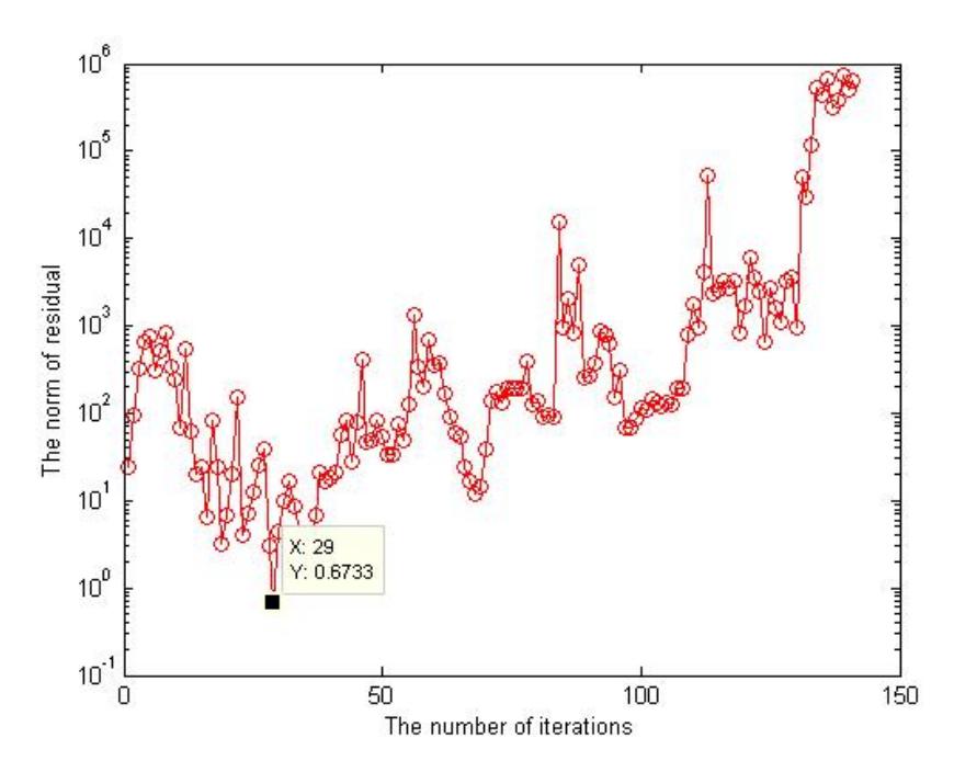
Figure 1 The behaviour of the residual norms of an SLE in 300 dimensions.
As in RLLastIt, RLMinRes is initialized as follows
\[\mathbf{x}_0 = \mathbf{x}_m,\tag{20}\] and y as in Eq. (16). If we repeat this step, we will find a good approximate solution as explained previously. The procedures of LMinRes and RLMinRes are presented in Algorithm 2 and Algorithm 3 respectively.
Algorithm 2 The LMinRes Algorithm.
- 1. Fix the number of iterations to, say, k, and the tolerance, \(\epsilon\), to 1E-13.
- 2. Collect all k iterates as in Eq. (17).
- 3. Collect all of the residual norms as in Eq. (18).
- 4. Compute the minimum values as in Eq. (19) and specify the index of the minimum value as m.
- 5. Obtain the approximate solution as well as the residual norm as follows
\[sol_{min} = data_{sol}(m), (21)\]
\[norm_{min} = \|\mathbf{r}_m\|. \tag{22}\]
6. Stop.
Algorithm 3 TheRLMinRes algorithm.
- 1. Initialize a Lanczos-type algorithm with initial guesses \(\mathbf{x}_0\) and \(\mathbf{y}\).
- 2. Run LMinRes algorithm for k iterations and obtain \(sol_{min}\) and \(norm_{min}\).
- 3. while \(norm_{min} \geq \epsilon\) do
- i. \(\mathbf{x} = sol_{min}\),
- ii. \(\mathbf{y} = \mathbf{b} A \mathbf{x}\).
- 4. Run LMinRes algorithm for k iterations.
- 5. endwhile.
- 6. Take \(sol_{min}\) as the approximate solution.
- 7. Stop.
3.3 Restarting Lanczos-type Algorithms with the Vector of Median Values
Consider again relations Eq. (17) and Eq. (18). For each \(x_i\), i=1,2,...,n, we set
\[w_{1} = \left\{ x_{1}^{(1)}, x_{2}^{(1)}, \cdots, x_{k}^{(1)} \right\}\] \[w_{2} = \left\{ x_{1}^{(2)}, x_{2}^{(2)}, \cdots, x_{k}^{(2)} \right\}\] \[\vdots\] \[w_{n} = \left\{ x_{1}^{(n)}, x_{2}^{(n)}, \cdots, x_{k}^{(n)} \right\}\] (23)
where \(w_i\) is arranged such that it consists of the \(i^{th}\) entry of each vector \(\mathbf{x}_i\), for i=1,2,...,n. For instance, \(w_1\) is the set of all of the first entries of the iterates, \(w_2\) is the set of all of the second entries of the iterates, etc. Thus, if we calculate the mean, median, and mode values of each \(w_i\) and we use them as the first entry, the second entry, etc... of a vector, it leads to a new vector solution. In other words, the new vector contains the values of either mean, median, or mode of all the first entries, the second entries, etc... of all the iterates. Our investigation of these entries showed that the best results are obtained with the median values. The approximate solution based on the median values of entries is as follows,
\[\mathbf{x}_{med} = \begin{bmatrix} x_1^{med} \\ x_2^{med} \\ \vdots \\ x_n^{med} \end{bmatrix}\] (24)
and \(x_i^{med} = med \{w_i\}\), for i = 1, 2, ..., n.
The procedure described above for creating an approximate solution from the median values of the entries of iterates generated by the Lanczos-type algorithm used is presented in algorithmic form as Algorithm 4 or LMedVal.
Algorithm 4 The LMedVal algorithm.
- 1. Initialize a Lanczos-type algorithm with initial guesses \(\mathbf{x}_0\) and \(\mathbf{y}\). Run it for k iterations
- 2. Collect all of k iterates as in Eq. (17).
- 3. for i = 1, 2, ..., n
- 4. Set \(w_i\) as in Eq. (23)
- 5. Compute the median value of the entries of each \(w_i\) as follows \(med(i) = median(w_i)\).
- 6. endfor
- 7. Compute the approximate solution as follows
\[\mathbf{x}_{med} = med(1:n)^T\]
8. Compute the residual norm of the solution as follows
\[res_{med} = \mathbf{b} - A \mathbf{x}_{med},\]
\(norm\_med = norm(res_{med}).\)
9. Stop
The procedure described above to restart the Lanczos-type algorithm from the output of LMedVal is presented in algorithmic form as Algorithm 5 or RLMedVal. Its initialization is as follows,
\[\mathbf{x}_0 = \mathbf{x}_{med},\tag{25}\] and vector \(\mathbf{y}\) as in Eq. (16), where \(\mathbf{x}_{med}\) as in Eq. (24).
Algorithm 5 TheRLMedVal algorithm
- 1. Fix the number of iterations to k and the tolerance \(\epsilon\) to 1E-13.
- 2. Run LMedVal for k iterations and obtain \(sol_{med}\) as well as \(norm_{med}\).
- 3. while \(norm_{med} \ge \epsilon\) do
- i. \(\mathbf{x} = \mathbf{x}_{med}\),
- ii. \(\mathbf{y} = \mathbf{b} A\mathbf{x}\).
- 4. Run LMedVal for k iterations.
- 5. endwhile.
- 6. Take \(sol_{med}\) as the approximate solution.
- 7. Stop.
3.4 The Theoretical Point of View
Suppose we solve an SLE using RLLastIt. Denote \(x_k^{(j)}\), j=1,2,...,s, and s>0 integer, as the \(k^{th}\) iterate of the \(j^{th}\) run of a Lanczos-type algorithm. In other words, s is the number of cycles of RLLastIt. Assume that the residual norm of the first cycle is greater than the convergence tolerance, i.e.
\[\left\|\mathbf{r}_{k}^{(1)}\right\| > \epsilon_{1},\tag{26}\] for some \(\epsilon_1 > 0\). Obviously, if this is not the case, the algorithm would have stopped with an acceptable approximate solution. Consider the results of Section 3.1 and by the definition of the Krylov subspace given in Section 2.1, iterate
\(\mathbf{x}_k^{(2)}\) of the second cycle of RLLasIt satisfies the following two conditions:
\[\mathbf{x}_{k}^{(2)} - \mathbf{x}_{0} \in K_{k}(A, \mathbf{r}_{0}),\] (27)
\[\mathbf{r}_k^{(2)} = \mathbf{b} - A \mathbf{x}_k^{(2)} \perp K_k(A^T, \mathbf{y}), \tag{28}\] where \({\bf r}_0 = {\bf r}_k^{(1)}\).
Substitute Eq. (15) into Eq. (27) to get:
\[\mathbf{x}_{k}^{(2)} - \mathbf{x}_{k}^{(1)} \in K_{k}\left(A, \mathbf{r}_{k}^{(1)}\right).\] (29)
Following the results in Eq. (5), we have:
\[\mathbf{r}_{k}^{(2)} = \mathbf{r}_{k}^{(1)} + \alpha_{1} A \mathbf{r}_{k}^{(1)} + \alpha_{2} A^{2} \mathbf{r}_{k}^{(1)} + \dots + \alpha_{k} A^{k} \mathbf{r}_{k}^{(1)}\] \[= P_{k}(A) \mathbf{r}_{k}^{(1)}, \tag{30}\] where \(P_k(A) = 1 + \alpha_1 A + \cdots + \alpha_k A^k\).
Calculating the norm of \(\mathbf{r}_k^{(2)}\) in Eq. (30) yields
\[\left\| \mathbf{r}_{k}^{(2)} \right\| = \left\| P_{k}(A)\mathbf{r}_{k}^{(1)} \right\|\] \[\leq \left\| P_{k}(A) \right\| \left\| \mathbf{r}_{k}^{(1)} \right\|. \tag{31}\]
If this residual norm is still bigger than the tolerance \(\epsilon_1\), we restart again, in which case we will have the third cycle, giving
\[\mathbf{r}_k^{(3)} = P_k(A)\mathbf{r}_k^{(2)}.\] (32)
Calculating the norm of \(\mathbf{r}_k^{(3)}\) as
\[\|\mathbf{r}_{k}^{(3)}\| = \|P_{k}(A)\mathbf{r}_{k}^{(2)}\|\] \[\leq \|P_{k}(A)\| \|\mathbf{r}_{k}^{(2)}\| \leq \|P_{k}(A)\|^{2} \|\mathbf{r}_{k}^{(1)}\|, \text{ from Eq. (31) (33)}\]
If this procedure is continued, then for the \(s^{th}\) cycle we have:
\[\|\mathbf{r}_{k}^{(s)}\| = \|P_{k}(A)\mathbf{r}_{k}^{(s-1)}\| \le \|P_{k}(A)\|^{s} \|\mathbf{r}_{k}^{(1)}\|\] (34)
From Eq. (31), Eq. (33), and Eq. (34), and since \(||P_k(A)|| > 0\), we conclude that
\[\left\|\mathbf{r}_{k}^{(s)}\right\| \leq \left\|\mathbf{r}_{k}^{(s-1)}\right\| \leq \cdots \left\|\mathbf{r}_{k}^{(1)}\right\| \tag{35}\] where \(s \ge 1\) is the number of cycles. This leads to the following result:
Theorem 1 Suppose we solve an SLE using a Lanczos-type algorithm. Let \(x_k^{(1)}\) be the last iterate generated by this algorithm after k iterations. Given a tolerance \(\epsilon > 0\), we assume that the associated residual norm \(\|r_k^{(1)}\| > \epsilon\). Restarting the algorithm with \(x_k^{(1)}\) allows it to generate an iterate with a better residual norm than those of the previous iterates.
Practically, breakdown may still occur between cycles, which causes the algorithm to stop before reaching a good approximate solution. We cannot guarantee that a breakdown will not occur in the first cycle, or any cycle for that matter.
4 Numerical Results and Discussion
We solved different size problems ranging from dimension 1000 to 70000. The test problems were carried out in MatLab 2012b using two different systems, Windows with processor RAM 6GB for solving the medium-scale problems, and Unix0 with 256 GB for solving the large-scale problems. We implemented the RLLastIt, RLMinRes, and RLMedVal algorithms, as well as other supporting procedures such as LMedVal. The experiments were carried out via Algorithm 6, which calls RLLastIt, RLMinRes, RLMedVal.
Algorithm 6 Restarting Lanczos-type algorithms from three different points.
- 1. Fix the number of iterations to k and the tolerance \(\epsilon\) to 1E-13.
- 2. Run RLLastIt, RLMinRes, RLMedVal for k iterations.
- 3. WHILE \(norm_{last} \ge \epsilon\) do
- 4. Run RLLastIt for k iterations.
- 5. Run RLMinRes for k iterations.
- 6. Run RLMedVal for k iterations.
- 7. ENDWHILE.
- 8. Take \(l_{last}\), \(sol_{min}\) and \(sol_{med}\) as the approximate solution of each above algorithm, respectively.
- 9. Stop.
We solve several systems of linear equations \(A\mathbf{x} = \mathbf{b}\), with matrix A being of the form
\[A = \begin{pmatrix} B & -I & \cdots & \cdots & 0 \\ -I & B & -I & \cdots & \cdots \\ \vdots & \ddots & \ddots & \ddots & \vdots \\ & & -I & B & -I \\ 0 & \cdots & \cdots & -I & B \end{pmatrix}\] \[(36)\] where
\[B = \begin{pmatrix} 4 & \alpha & \cdots & \cdots & 0 \\ \beta & 4 & \alpha & \cdots & \cdots \\ \vdots & \ddots & \ddots & \ddots & \vdots \\ & \beta & 4 & \alpha \\ 0 & \cdots & \cdots & \beta & 4 \end{pmatrix}\](37)
with \(\alpha = -1 + \delta\), \(\beta = -1 - \delta\), and \(\delta\) takes values 0.0, 0.2, 0.5, 0.8, 5.0, and 8.0. Matrix A is the result of the descritization of a linear differential operator [1]. We use the Orthodir algorithm, or Algorithm 7, in this experiment as a representative of Lanczos-type algorithms. We also use 100 iterations to make up a cycle, which means that the intermediate solution is found after 100 iterations.
Algorithm 7 Orthodir Algorithm [12].
- 1. Initialization. Choose \(\mathbf{x}_0\) and \(\mathbf{y}_0\). Set \(\mathbf{x}=\mathbf{x}_0\), \(\mathbf{r}_0=\mathbf{b}-A\mathbf{x}_0\), \(\mathbf{y}_0=\mathbf{y}\), and \(\mathbf{z}_0=\mathbf{r}_0\).
- 2. for k = 0,1,2,... do
- 3. \(\mathbf{y}_k = A^T \mathbf{y}_k 1\)4. \(A_{k+1} = \frac{\langle -\mathbf{y}_k | \mathbf{r}_k \rangle}{\langle \mathbf{y}_k | A \mathbf{z}_k \rangle}\)
- 5. \(\mathbf{x}_{k+1} = \mathbf{x}_k A_{k+1} \mathbf{z}_k\).
- 6. \(\mathbf{r}_{k+1} = \mathbf{r}_{k} + A_{k+1} A \mathbf{z}_{k}.\)
- 7. Run RLMedVal for k iterations.
- 8. end for
- 9. \(sol_{last} = \mathbf{x}_k\).
- 10. \(norm_{last} = ||\mathbf{r}_k||\).
- 11. Stop.
Table 1 Results of RLLastIt, RLMinRes, and RLMedVal on problems with = 0.0.
| Dim | RLLastIt | RLMinRes | RLMedVal | |||||||
|---|---|---|---|---|---|---|---|---|---|---|
| n | ‖𝐫𝒌‖ | T (s) | cycles | ‖𝐫𝒎𝒊𝒏‖ | T (s) | cycles | ‖𝐫𝒎𝒆𝒅‖ | T (s) | cycles | |
| 1000 | 5.7290E-14 | 2.0159 | 16 | 7.4630E-14 | 1.1293 | 11 | 7.7686E-14 | 1.9818 | 12 | |
| 2000 | NaN | NA | NA | 7.9179E-14 | 3.5393 | 10 | 7.2049E-14 | 5.1083 | 8 | |
| 3000 | NaN | NA | NA | 7.1515E-14 | 8.0831 | 10 | 9.2942E-14 | 10.2765 | 12 | |
| 4000 | 6.6150E-14 | 34.3719 | 24 | 7.1737E-14 | 12.2651 | 9 | 9.7700E-14 | 17.8791 | 12 | |
| 5000 | 5.3701E-14 | 79.1186 | 36 | 6.8902E-14 | 18.5584 | 9 | 7.9847E-14 | 24.7685 | 12 | |
| 6000 | NaN | NA | NA | 7.1850E-14 | 25.8040 | 9 | 7.4920E-14 | 101.59 | 9 | |
| 7000 | NaN | NA | NA | 7.9874E-14 | 37.3090 | 12 | 7.4949E-14 | 50.6792 | 12 | |
| 8000 | 9.0251E-14 | 67.9472 | 14 | 6.7684E-14 | 45.5536 | 9 | NaN | NA | NA | |
| 9000 | 6.0401E-14 | 161.2933 | 24 | 7.0927E-14 | 63.9086 | 10 | 8.5236E-14 | 70.1496 | 11 | |
| 10000 | 6.6456E-14 | 165.7143 | 20 | 8.1881E-14 | 79.8814 | 10 | 8.5545E-14 | 93.5818 | 11 | |
| 20000 | 7.2688E-14 | 1285.5 | 40 | 7.4526E-14 | 318.159 | 10 | 9.9168E-14 | 1.2345E+03 | 12 | |
| 30000 | NaN | NA | NA | 7.9381E-14 | 2.2848E+04 | 9 | NaN | NA | NA | |
| 40000 | 9.5703E-14 | 1.9798E+04 | 47 | 8.0789E-14 | 9.5895E+04 | 13 | NaN | NA | NA | |
| 50000 | 202.3106 | 1.7797E+04 | 10 | 8.5386E-14 | 1.5375E+04 | 10 | NaN | NA | NA | |
| 60000 | 0.0014 | 2.6531E+04 | 10 | 7.5384E-14 | 2.1178E+04 | 10 | NaN | NA | NA | |
| 70000 | 3.8427E-08 | 5.0351E+04 | 15 | 9.2520E-14 | 3.0739E+04 | 10 | 8.4645E-14 | 6.4255E+04 | 15 | |
Table 2 Results of RLLastIt, RLMinRes, and RLMedVal on problems with = 0.2.
| Dim | RLLastIt | RLMinRes | RLMedVal | |||||||
|---|---|---|---|---|---|---|---|---|---|---|
| n | ‖𝐫𝒌‖ | T (s) | cycles | ‖𝐫𝒎𝒊𝒏‖ | T (s) | cycles | ‖𝐫𝒎𝒆𝒅‖ | T (s) | cycles | |
| 1000 | 6.5481E-14 | 2.0260 | 16 | 8.0389E-14 | 0.8079 | 7 | 7.7606E-14 | 1.9484 | 8 | |
| 2000 | 3.3041E-14 | 5.7515 | 14 | 1.2429E-13 | 7.6131 | 14 | 7.9129E-14 | 6.750 | 8 | |
| 3000 | NaN | NA | NA | 8.7363E-14 | 6.9168 | 8 | NaN | NA | NA | |
| 4000 | 4.0211E-14 | 23.8768 | 16 | 7.9746E-14 | 9.8956 | 7 | NaN | NA | NA | |
| 5000 | NaN | NA | NA | 5.1093E-14 | 17.1567 | 9 | NaN | NA | NA | |
| 6000 | 3.3399E-14 | 49.6966 | 15 | 7.0909E-14 | 21.6026 | 7 | 6.4865E-14 | 45.8989 | 9 | |
| 7000 | 5.4049E-14 | 76.8363 | 17 | 7.3018E-14 | 34.2061 | 8 | 8.6172E-14 | 68.6571 | 10 | |
| 8000 | NaN | NA | NA | 8.0677E-14 | 35.2509 | 7 | 7.8672E-14 | 71.3026 | 8 | |
| 9000 | 5.0507E-14 | 152.2841 | 21 | 6.6680E-14 | 48.2827 | 7 | 8.9150E-14 | 106.9637 | 8 | |
| 10000 | 5.6855E-14 | 205.5778 | 25 | 6.3812E-14 | 61.9360 | 8 | 8.2954E-14 | 118.8027 | 8 | |
| 20000 | NaN | NA | NA | 7.4526E-14 | 318.1595 | 10 | NaN | NA | NA | |
| 30000 | 9.7800E-14 | 1.1635E+04 | 50 | 6.7992E-14 | 3.11E+03 | 9 | 7.6804E-14 | 7.12E+03 | 10 | |
| 40000 | NaN | NA | NA | 5.9208E-14 | 6.16E+03 | 8 | NaN | NA | NA | |
| 50000 | 9.9120E-14 | 3.6563E+04 | 75 | 7.4136E-14 | 7.38E+03 | 8 | 9.8225E-14 | 1.36E+04 | 10 | |
| 60000 | 9.9668E-14 | 2.5750E+04 | 44 | 8.3763E-14 | 9.68E+03 | 7 | 8.5780E-14 | 2.31E+04 | 11 | |
| 70000 | 1.5299E+03 | 5.5568E+04 | 10 | 7.1895E-14 | 1.56E+04 | 8 | 9.2065E-14 | 2.74E+04 | 10 | |
Table 3 Results of RLLastIt, RLMinRes, and RLMedVal on problems with = 0.5.
| Dim | RLLastIt | RLMinRes | RLMedVal | |||||||
|---|---|---|---|---|---|---|---|---|---|---|
| n | ‖𝐫𝒌‖ | T (s) | cycles | ‖𝐫𝒎𝒊𝒏‖ | T (s) | cycles | ‖𝐫𝒎𝒆𝒅‖ | T (s) | cycles | |
| 1000 | NaN | NA | NA | 6.7241E-14 | 0.4985 | 6 | 8.0317E-14 | 0.9676 | 6 | |
| 2000 | 6.6028E-14 | 3.0730 | 8 | 7.1644E-14 | 1.6560 | 5 | NaN | NA | NA | |
| 3000 | 2.0914E-14 | 6.1322 | 8 | 2.9349E-14 | 3.7583 | 5 | 8.2315E-14 | 5.5742 | 7 | |
| 4000 | 4.0636E-14 | 10.5073 | 8 | 8.5704E-14 | 6.8387 | 5 | 7.3850E-14 | 8.6492 | 6 | |
| 5000 | 5.3701E-14 | 13.8288 | 7 | 8.7432E-14 | 9.4709 | 5 | 6.6026E-14 | 13.3348 | 7 | |
| 6000 | 4.0015E-14 | 14.3912 | 8 | 4.4088E-14 | 13.5595 | 5 | 7.9435E-14 | 19.0317 | 7 | |
| 7000 | 7.6507E-14 | 28.4045 | 7 | 6.1367E-14 | 19.8723 | 5 | 9.3416E-14 | 23.4865 | 7 | |
| 8000 | 7.6507E-14 | 46.6633 | 9 | 6.7684E-14 | 24.9942 | 5 | 7.3388E-14 | 23.4865 | 7 | |
| 9000 | 2.0877E-14 | 47.3239 | 10 | 8.1464E-14 | 32.4579 | 6 | 7.5110E-14 | 43.3506 | 6 | |
| 10000 | NaN | NA | NA | 7.6418E-14 | 36.7934 | 5 | NaN | NA | NA | |
| 20000 | NaN | NA | NA | 5.5184E-14 | 171.5886 | 6 | 7.9658E-14 | 164.7378 | 6 | |
| 30000 | 3.0472E-14 | 456.2760 | 8 | 8.3265E-14 | 435.3542 | 6 | 8.6487E-14 | 438.9958 | 6 | |
| 40000 | 9.1562E-14 | 1.3454E+04 | 18 | 7.6668E-14 | 4.95E+03 | 6 | 8.5023E-14 | 10546.413 | 7 | |
| 50000 | 7.5725E-14 | 1.3499E+03 | 12 | 8.0480E-14 | 9.21E+03 | 5 | 8.8901E-14 | 17177.462 | 7 | |
| 60000 | 9.5620E-14 | 17342.312 | 20 | 7.8496E-14 | 9.69E+03 | 6 | 8.1470E-14 | 1.55E+03 | 6 | |
| 70000 | 9.8198E-14 | 3.3085E+04 | 25 | 6.9337E-14 | 1.19E+04 | 7 | 8.2264E-14 | 2.32E+04 | 7 | |
Table 4 Results of RLLastIt, RLMinRes, and RLMedVal on problems with = 0.8.
| Dim | RLLastIt | RLMinRes | RLMedVal | ||||||
|---|---|---|---|---|---|---|---|---|---|
| n | ‖𝐫𝒌‖ | T (s) | cycles | ‖𝐫𝒎𝒊𝒏‖ | T (s) | cycles | ‖𝐫𝒎𝒆𝒅‖ | T (s) | cycles |
| 1000 | 4.6646E-14 | 0.3958 | 4 | 1.2362E-13 | 0.4031 | 4 | 1.9188E-13 | 0.5585 | 4 |
| 2000 | 9.0517E-14 | 2.7572 | 6 | 7.1644E-14 | 1.6560 | 6 | 6.2576E-14 | 3.0358 | 6 |
| 3000 | 5.2252E-14 | 3.5538 | 5 | 9.9039E-14 | 2.7697 | 4 | 9.1631E-14 | 3.4874 | 5 |
| 4000 | 5.1236E-14 | 6.2464 | 5 | 5.0994E-14 | 4.8783 | 5 | 8.4532E-14 | 6.1081 | 6 |
| 5000 | 2.6627E-14 | 9.3331 | 5 | 4.6503E-14 | 6.4221 | 4 | 7.5342E-14 | 8.7590 | 6 |
| 6000 | 4.0015E-14 | 14.3912 | 5 | 1.5693E-14 | 13.8603 | 5 | 8.5979E-14 | 14.7563 | 5 |
| 7000 | NaN | NA | NA | 6.4924E-14 | 15.4388 | 5 | NaN | NA | NA |
| 8000 | NaN | NA | NA | 4.8607E-14 | 25.5804 | 5 | 6.8697E-14 | 24.2593 | 7 |
| 9000 | 7.2386E-14 | 32.2374 | 5 | 6.9432E-14 | 28.7406 | 4 | 8.7765E-14 | 27.7122 | 5 |
| 10000 | 4.4203E-14 | 40.7000 | 5 | 5.8453E-14 | 30.8759 | 5 | 9.5466E-14 | 35.9651 | 6 |
| 20000 | 3.3223E-14 | 159.2071 | 5 | 6.9427E-14 | 117.3181 | 4 | 8.1042E-14 | 133.124 | 5 |
| 30000 | NaN | NA | NA | 8.5189E-14 | 408.2613 | 6 | NaN | NA | NA |
| 40000 | 9.3120E-14 | 3.4339E+03 | 14 | 9.9397E-14 | 3.8403E+03 | 5 | 9.7811E-14 | 6.969E+03 | 4 |
| 50000 | 7.3387E-14 | 3.9644E+03 | 6 | 8.0193E-14 | 4.3404E+03 | 4 | 8.3000E-14 | 7.910E+03 | 6 |
| 60000 | 7.7921E-14 | 1.295E+04 | 8 | 9.4813E-14 | 7.5053E+03 | 4 | 8.0392E-14 | 7.492E+03 | 6 |
| 70000 | 8.4024E-14 | 1.902E+04 | 8 | 7.8985E-14 | 9.986E+04 | 4 | 7.5368E-14 | 1.329E+04 | 5 |
Table 5 Results of RLLastIt, RLMinRes, and RLMedVal on problems with = 5.
| Dim | RLLastIt | RLMinRes | RLMedVal | ||||||
|---|---|---|---|---|---|---|---|---|---|
| n | ‖𝐫𝒌‖ | T (s) | cycles | ‖𝐫𝒎𝒊𝒏‖ | T (s) | cycles | ‖𝐫𝒎𝒆𝒅‖ | T (s) | cycles |
| 1000 | 6.6783E-13 | 0.8566 | 9 | 1.1544E-13 | 0.7058 | 9 | 7.5428E-14 | 0.9535 | 9 |
| 2000 | 9.0517E-14 | 2.4700 | 9 | 1.6451E-13 | 2.1698 | 9 | 4.3856E-14 | 3.0832 | 9 |
| 3000 | 8.9938E-14 | 6.1439 | 8 | 1.1733E-13 | 5.2819 | 8 | 5.1801E-14 | 6.3681 | 8 |
| 4000 | 2.0649E-13 | 6.2464 | 6 | 1.4507E-13 | 8.6705 | 6 | 9.6175E-14 | 12.1345 | 6 |
| 5000 | 2.0727E-13 | 9.8154 | 8 | 1.3336E-13 | 12.3384 | 8 | 8.6350E-14 | 14.3220 | 7 |
| 6000 | 9.1796E-14 | 16.0040 | 10 | 2.1285E-13 | 19.3882 | 10 | 7.6867E-14 | 14.7563 | 7 |
| 7000 | 9.2341E-14 | 21.2654 | 13 | 1.1998E-13 | 29.0991 | 13 | 9.6799E-14 | 21.5071 | 7 |
| 8000 | 9.4310E-14 | 32.1371 | 12 | 1.1228E-13 | 37.4504 | 12 | 9.4843E-14 | 28.639 | 7 |
| 9000 | 9.9740E-13 | 32.2374 | 10 | 1.1051E-13 | 40.1467 | 10 | 9.9463E-14 | 41.8971 | 6 |
| 10000 | 1.0468E-13 | 43.2287 | 13 | 1.2264E-13 | 71.6121 | 13 | 8.6507E-14 | 45.5433 | 6 |
| 20000 | 9.8099E-14 | 45.5492 | 183 | 1.8305E-13 | 758.8923 | 183 | 9.2670E-14 | 74.9466 | 7 |
| 30000 | 2.5585E-13 | 81.2740 | 8 | 1.3291E-13 | 475.0696 | 8 | 9.3863E-14 | 222.3481 | 8 |
| 40000 | 1.6819E-12 | 785.5109 | 10 | 1.3931E-13 | 4.4190E+03 | 10 | 9.4113E-14 | 532.888 | 8 |
| 50000 | 1.3379E-12 | 594.4041 | 12 | 1.5053E-13 | 1.2285E+04 | 12 | 9.5873E-14 | 8213.771 | 10 |
| 60000 | 1.5239E-12 | 5486.982 | 12 | 1.5722E-13 | 1.238E+04 | 12 | 9.9868E-14 | 20937.43 | 12 |
| 70000 | 1.2905E-12 | 1.161E+04 | 13 | 1.5767E-13 | 2.6015E+04 | 13 | 9.8246E-14 | 23439.0 | 13 |
Table 6 Results of RLLastIt, RLMinRes, and RLMedVal on problems with = 8.
| Dim | RLLastIt | RLMinRes | RLMedVal | |||||||
|---|---|---|---|---|---|---|---|---|---|---|
| n | ‖𝐫𝒌‖ | T (s) | cycles | ‖𝐫𝒎𝒊𝒏‖ | T (s) | cycles | ‖𝐫𝒎𝒆𝒅‖ | T (s) | cycles | |
| 1000 | 9.4847E-14 | 0.8644 | 12 | 1.4204E-13 | 0.7227 | 12 | 7.5478E-14 | 2.0025 | 9 | |
| 2000 | 9.7642E-14 | 3.2058 | 18 | 1.2579E-13 | 2.8480 | 9 | 6.2576E-14 | 2.8289 | 9 | |
| 3000 | 1.8544E-13 | 7.3663 | 9 | 1.2535E-13 | 5.7008 | 9 | 7.6937E-14 | 6.4005 | 9 | |
| 4000 | 2.6912E-13 | 9.8464 | 9 | 1.0890E-13 | 9.8928 | 9 | 9.6175E-14 | 11.1164 | 9 | |
| 5000 | 2.1612E-13 | 18.2973 | 9 | 1.5348E-13 | 15.7859 | 9 | 8.2624E-14 | 16.1618 | 9 | |
| 6000 | 2.4049E-13 | 26.4696 | 9 | 1.8742E-13 | 20.8982 | 9 | 8.7058E-14 | 23.6583 | 9 | |
| 7000 | 3.8371E-13 | 33.9227 | 9 | 1.1998E-13 | 30.0858 | 8 | 9.4308E-14 | 32.8377 | 9 | |
| 8000 | 1.0312E-13 | 41.5876 | 8 | 1.4894E-13 | 39.6557 | 10 | 9.8204E-14 | 42.3492 | 8 | |
| 9000 | 2.9206E-13 | 55.3891 | 10 | 1.4201E-13 | 50.4974 | 9 | 8.5654E-14 | 57.2675 | 10 | |
| 10000 | 3.3040E-13 | 69.0426 | 9 | 1.5087E-13 | 62.4519 | 11 | 8.6507E-14 | 62.4430 | 9 | |
| 20000 | 3.9022E-13 | 276.9322 | 11 | 1.4875E-13 | 259.4267 | 6 | 9.8224E-14 | 288.0455 | 11 | |
| 30000 | NaN | NA | NA | 8.5189E-14 | 408.2613 | 8 | 9.3115E-14 | NA | NA | |
| 40000 | 12629.47 | 12629.417 | 20 | 1.6024E-13 | 6.249E+03 | 20 | NaN | 7.236E+03 | 20 | |
| 50000 | 8.5401E-13 | 33035.391 | 26 | 1.0820E-13 | 1.696E+04 | 26 | 9.9614E-14 | 1.4038+04 | 26 | |
| 60000 | 1.3279E-12 | 32253 | 7 | 1.1333E-13 | 1.722E+04 | 7 | 9.9792E-14 | 2.0937E+04 | 7 | |
| 70000 | 1.2417E-13 | 53545.694 | 10 | 3.9254E-13 | 2.652E+04 | 6 | 5.4308E-13 | 2.0694E+04 | 7 | |
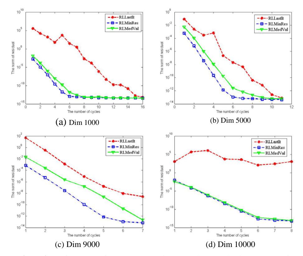
Figure 2 Performance of RLLastIt, RLMinRes, and RLMedVal on SLE's of several dimensions, for δ = 0.2.
4.1 Discussion
We consider two cases, (i) the cases with δ = 0.0, δ = 0.2, δ = 0.5, and δ = 0.8, leading to SLE's with matrices A having condition numbers 119.9999, 98.6081, 62.2227, and 44.3210, respectively; (ii) the cases with δ = 5 and δ = 8, leading to SLE's with matrices A having condition numbers 27.4932 and 24.4970, respectively. Note that the matrices of case (i) have slightly larger condition numbers compared to those of case (ii). However, according to [17-19], the systems are categorized as well-conditioned.
For the first case, RLMinRes has the best performance in terms of accuracy and stability compared to RLLastIt and RLMedVal. As can be seen in Table 1, RLMinRes consistently meets the tolerance when solving several problems. In fact, it is also more robust than RLLastIt and RLMedVal, where there is no breakdown. These results are similar to those of Tables 2, 3 and 4, where they are related to the cases of = 0.2 , = 0.5, and , = 0.8 respectively. For the second case, the results of which are in Tables 5 and 6, RLMedVal is more accurate than RLMinRes, though it is slower. The worst performance in both cases is that of RLLastIt. In fact, it still suffers from breakdown. The behaviour of the restarting from three different points is represented in Figure 2.
5 Summary
In this study we have discussed restarting Lanczos-type algorithms from three different, reasonable points to combat breakdown when solving SLE's. Algorithms called RLLastIt, RLMinRes, and RLMedVal, corresponding to the three different restartings, have been implemented. The numerical results point to restarting from the iterate with lowest residual norm, i.e. RLMinRes, as the most successful. Restarting from the iterate whose entries are the median values of the entries of previous iterates, i.e. alorithm RLMedVal, is sometimes more robust than RLMinRes. Restarting from the last iterate, or RLLastIt, is the worst in both cases. These results confirm our intuitive assessment of each case. For instance, restarting from the best approximate solution found so far, as in RLMinRes, should perform well. And it does indeed. Note that we have solved problems with dimension up to 70000. These are not trivial problems to solve numerically with any method. Moreover, Lanczos-type algorithms can't solve them without restarting or switching.
Interesting questions following from this work could be to investigate whether the quality of the Krylov subspace in which approximate solutions are generated can be estimated from the starting point. Is there any way to tell whether one Krylov subspace is better than another? Can the length of the cycle be determined accurately to avoid stopping too early before breakdown? These issues are relevant in other contexts too and certainly in the context of switching.
Acknowledgements
This project is supported by the Indonesian Government through the Directorate General of Higher Education (DIKTI) Scholarship 2010.