
1 Introduction
A delay process in a metabolic system may represent the time necessary for a certain enzyme to actively start getting involved in a kinetic reaction. In our previous work [1], a mathematical model of the ethanol fermentation process by a single yeast cell was derived that took into consideration the effect of a delay in a certain reaction process and led to a system of delay differential equations. Numerical simulations by means of the Runge-Kutta method for a delay differential system were then used to approximate the transient behavior of the system. In the present work, we extend our study to approximate solutions analytically by using the matrix Lambert function to simulate the linearized delay differential system.
The Lambert function method was first applied by Wright [2] to analyze a linear delay differential system. The method was then improved by other researchers, such as Asl and Ulsoy [3], Ulsoy [4], and Nelson, et al. [5]. Here, we apply the method to generate the analytic solution of our system of which it is extremely difficult to find its closed form. This is due to the existence of a special transcendental equation that has an infinite number of roots (see Ivanoviene and Rimas [6]). We also compare our present numerical approach to the numerical Runge-Kutta method.
This paper is organized as follows. First, we introduce the linearized delay differential system taken from Kasbawati, et al. [1]. Next, we derive the solution using the matrix Lambert method, generate numerical procedures for the Lambert solution and compare the present results with our previous results of the Runge-Kutta method. The paper is closed by summaries and concluding remarks.
2 Linearized Delay Differential System of a Microbial Fermentation Model
Ethanol fermentation by a yeast cell is a multi-enzymatic system that is viewed as a branched metabolic pathway (see Figure 1). In our previous work [1], we have constructed equations for the fermentation process and introduced a delay term in the conversion reaction. The delay term appeared due to the existence of a rate-limiting step in the fermentation pathway; time completion was needed by the enzyme to restore its active site.
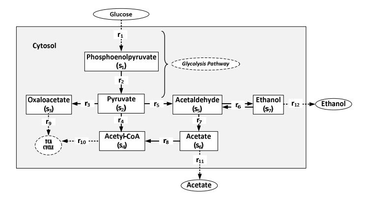
Figure 1 Reaction r1 refers to the rate of glucose supply, ri refers to the conversion reaction catalyzed by the following enzymes: 2: pyruvate kinase, 3: pyruvate carboxylase, 4: pyruvate dehydrogenase complex, 5: pyruvate decarboxylase, 6: alcohol dehydrogenase, 7: acetaldehyde dehydrogenase, 8: acetyl-CoA synthetase. TCA cycle is the tricarboxylic acid cycle. Single arrows indicate irreversible reaction while double arrows indicate reversible reaction [1].
By assuming that a discrete time delay took place at the first reaction kinetic equation (see \(r_2\) in Figure 1), the dimensionless delay differential equations are given by [1]:
\[\frac{dx_{1}(\overline{t})}{d\overline{t}} = \widetilde{G} - \frac{v_{1}x_{1}(\overline{t}-1)}{x(\overline{t}-1)+1},\] \[\frac{dx_{2}(\overline{t})}{d\overline{t}} = \frac{v_{1}x(\overline{t}-1)}{x_{1}(\overline{t}-1)+1} - \frac{v_{2}x_{2}(\overline{t})}{x_{2}(\overline{t})+K_{2}} - \frac{v_{3}x_{2}(\overline{t})}{x_{2}(\overline{t})+K_{3}} - \frac{v_{4}x_{2}(\overline{t})}{x_{2}(\overline{t})+K_{4}},\] \[\frac{dx_{3}(\overline{t})}{d\overline{t}} = \frac{v_{2}x_{2}(\overline{t})}{x_{2}(\overline{t})+K_{2}} - \sigma_{1}x_{3}(\overline{t}),\] \[\frac{dx_{4}(\overline{t})}{d\overline{t}} = \frac{v_{3}x_{2}(\overline{t})}{x_{2}(\overline{t})+K_{3}} + \frac{v_{7}x_{6}(\overline{t})}{x_{6}(\overline{t})+K_{7}} - \sigma_{2}x_{4}(\overline{t}),\] \[\frac{dx_{5}(\overline{t})}{d\overline{t}} = \frac{v_{4}x_{2}(\overline{t})}{x_{2}(\overline{t})+K_{4}} - \frac{v_{5f}K_{5b}X_{5}(\overline{t})-v_{5b}K_{5f}X_{7}(\overline{t})}{K_{5f}K_{5b}+K_{5f}X_{7}(\overline{t})} - \frac{v_{6}x_{5}(\overline{t})}{x_{5}(\overline{t})+K_{6}},\] \[\frac{dx_{6}(\overline{t})}{d\overline{t}} = \frac{v_{6}x_{5}(\overline{t})}{x_{5}(\overline{t})+K_{6}} - \frac{v_{7}x_{6}(\overline{t})}{x_{6}(\overline{t})+K_{7}} - \sigma_{3}x_{6}(\overline{t}),\] \[\frac{dx_{7}(\overline{t})}{d\overline{t}} = \frac{v_{5f}K_{5b}X_{5}(\overline{t})-v_{5b}K_{5f}X_{7}(\overline{t})}{K_{5f}K_{5b}+K_{5f}X_{7}(\overline{t})} - \sigma_{4}x_{7}(\overline{t}),\] \[\frac{dx_{7}(\overline{t})}{d\overline{t}} = \frac{v_{5f}K_{5b}X_{5}(\overline{t})-v_{5b}K_{5f}X_{7}(\overline{t})}{K_{5f}K_{5f}X_{7}(\overline{t})} - \sigma_{4}x_{7}(\overline{t}),\] with dimensionless variable and dimensionless time \(x_i = s_i / K_1\), \(\overline{t} = t / \tau\), dimensionless time delay \(\tilde{\tau} = 1\), and dimensionless parameters \((\forall i = 1, \dots, 4, j = 1, \dots, 7)\),
\[\tilde{G} = \frac{\tau G}{K_1}, V_j = \frac{\tau V_j}{K_1}, \ \kappa_j = \frac{\tau K_j}{K_1}, \ \kappa_{sf} = \frac{K_1}{K_s^f}, \ \kappa_{sb} = \frac{K_1}{K_s^b}, \ \sigma_i = \delta_i \tau.\]
The nomenclature is shown in Table 1. The reader can find detailed information concerning the model in Kasbawati, et al. [1].
Eq. (1) has only one steady state solution, defined as \(\mathbf{x}_E = (x_1^*, x_2^*, x_3^*, x_4^*, x_5^*, x_6^*, x_7^*)\), with
\[\vec{x}_{1} = \frac{\tilde{G}}{v_{1} - \tilde{G}}, \quad \vec{x}_{3} = \frac{v_{2}\vec{x_{2}}}{(\vec{x_{2}} + \kappa_{2})\sigma_{1}}, \quad \vec{x}_{4} = \frac{1}{\sigma_{1}} \left[ \frac{v_{3}\vec{x_{2}}}{(\vec{x_{2}} + \kappa_{3})} + \frac{v_{7}\vec{x_{6}}}{(\vec{x_{6}} + \kappa_{7})} \right], \quad \vec{x}_{5} = \frac{\kappa_{5f}\vec{x_{7}}(v_{5b} + \sigma_{4}[\kappa_{5b} + \vec{x_{7}}])}{\kappa_{5b}(v_{5f} - \sigma_{4}\vec{x_{7}})}.\] where \(X_2^*\), \(X_7^*\), and \(X_6^*\), respectively, are the roots of the cubic and quadratic polynomials (see [1]). Steady state \(\mathbf{X}_E\) will be positive if the following conditions are fulfilled:
\[\tilde{G} < V_1 < V_i\], \(i = 2, \dots, 4, \ V_4 < V_6 < (V_6 + V_{5f}), \ K_6 < K_{5f}\)
Table 1 Definitions of the normalized variables and parameters.
| Symbol | Definition |
|---|---|
| \(S_{i}\) | Concentration of metabolites (see Figure 1), g/l. |
| \(\delta_{_{i}}\) | Specific rate of product outflow, 1/h. |
| G | Rate of glucose supply, g/lh. |
| \(V_{_j}\) | Maximum reaction rate of enzymes, g/lh. |
| \(K_{j}\) | Michaelis constant of the enzymes (see Figure 1), which react irreversibly, g/l. |
| \(K_5^f\) | Michaelis constant of forward reaction of alcohol dehydrogenase, which reacts reversibly, g/l. |
| \(K_5^b\) | Michaelis constant of backward reaction of alcohol dehydrogenase, g/l. |
| \(\tau\) | Length of time required by enzyme pyruvate kinase to convert |
| phosphoenolpyruvate \((s_1)\) into pyruvate \((s_2)\). |
Linearizing Eq. (1) at equilibrium \(\mathbf{X}_E\), we obtain
\[\dot{\xi}(\overline{t}) = \mathbf{J}_1 \xi(\overline{t}) + \mathbf{J}_2 \xi(\overline{t} - 1). \tag{2}\] with \[\xi(\overline{t}) = (x(\overline{t}) - x_E)\], \(\xi(\overline{t} - 1) = (x(\overline{t} - 1) - x_E)\), \(J_1 = \begin{bmatrix} A & 0 \\ C & D \end{bmatrix}\), \(J_2 = \begin{bmatrix} A_d & 0 \\ 0 & 0 \end{bmatrix}\),
\[\mathbf{A} = \begin{bmatrix} 0 & 0 & 0 \\ 0 & -\sum_{i=2}^{4} \frac{V_{i} K_{i}}{(x_{2}^{*} + K_{i}^{*})^{2}} & 0 \\ 0 & \frac{V_{2} K_{2}}{(x_{2}^{*} + K_{2}^{*})^{2}} & -\sigma_{1} \end{bmatrix}, \ \mathbf{A}_{d} = \begin{bmatrix} -\frac{(V_{1} - \tilde{G})^{2}}{V_{1}} & 0 & 0 \\ \frac{(V_{1} - \tilde{G})^{2}}{V_{1}} & 0 & 0 \\ 0 & 0 & 0 & 0 \end{bmatrix}, \ \mathbf{C} = \begin{bmatrix} 0 & \frac{V_{3} K_{3}}{(x_{2}^{*} + K_{3}^{*})^{2}} & 0 \\ 0 & \frac{V_{4} K_{4}}{(x_{2}^{*} + K_{4}^{*})^{2}} & 0 \\ 0 & 0 & 0 \\ 0 & 0 & 0 \end{bmatrix},\]
\[\mathbf{D} = \begin{bmatrix} -\sigma_2 & 0 & \frac{V_6 K_6}{(x_6^* + K_6)^2} & 0 \\ 0 & -\left(\frac{V_5 K_5}{(x_5^* + K_5)^2} + \Delta_1\right) & 0 & \Delta_2 \\ 0 & \frac{V_5 K_5}{(S_5^* + K_5)^2} & -\left(\frac{V_6 K_6}{(x_6^* + K_6)^2} + \sigma_3\right) & 0 \\ 0 & \Delta_1 & 0 & -\left(\Delta_2 + \sigma_4\right) \end{bmatrix}\] \[\Delta_1 = \left(\frac{K_f K_b (K_b V_f + X_7^* [V_f + V_b])}{(K_b K_f + K_b X_5^* + K_f X_7^*)^2}\right), \ \Delta_2 = \left(\frac{K_f K_b (K_f V_b + X_5^* [V_f + V_b])}{(K_b K_f + K_b X_5^* + K_f X_7^*)^2}\right).\]
3 Solving the Linearized System Using the Lambert Function
Consider the linearized Eq. (2). Let the solution be written as
\[\xi(\overline{t}) = e^{S\overline{t}}\xi_0. \tag{3}\] where S is a \(7\times7\) matrix and \(\xi_0\) is a \(7\times1\) constant vector. Substituting Eq. (3) into Eq. (2) yields
\[\mathbf{S}e^{\mathbf{S}\overline{\tau}}\boldsymbol{\xi}_{0} - \mathbf{J}_{e}^{\mathbf{S}\overline{\tau}}\boldsymbol{\xi}_{0} - \mathbf{J}_{2}e^{\mathbf{S}(\overline{\tau}-1)}\boldsymbol{\xi}_{0} = \mathbf{0},\] \[\mathbf{S}e^{\mathbf{S}\overline{\tau}}\boldsymbol{\xi}_{0} - \mathbf{J}_{1}e^{\mathbf{S}\overline{\tau}}\boldsymbol{\xi}_{0} - \mathbf{J}_{2}e^{-\mathbf{S}}e^{\mathbf{S}\overline{\tau}}\boldsymbol{\xi}_{0} = \mathbf{0},\] \[(\mathbf{S} - \mathbf{J}_{1} - \mathbf{J}_{2}e^{-\mathbf{S}})e^{\mathbf{S}\overline{\tau}}\boldsymbol{\xi}_{0} = \mathbf{0}.\]
Since \(e^{S_1}\xi_0 \neq 0\), then for any arbitrary \(\xi_0 \neq 0\), we have
\[(\mathbf{S} - \mathbf{J}_{\perp}) = \mathbf{J}_{\perp} e^{-\mathbf{S}} \,. \tag{4}\]
Multiplying both sides of Eq. (4) by \(e^{s}e^{-J_{1}}\) gives
\[(\mathbf{S} - \mathbf{J}_1)e^{\mathbf{S}}e^{-\mathbf{J}_1} = \mathbf{J}_2e^{-\mathbf{J}_1}.\] (5)
Since \(J_1J_2 \neq J_2J_1\), then \(SJ_1 \neq J_1S\). Therefore we have
\[(\mathbf{S} - \mathbf{J}_1)e^{\mathbf{S}}e^{-\mathbf{J}_1} \neq (\mathbf{S} - \mathbf{J}_1)e^{(\mathbf{S} - \mathbf{J}_1)}\] (6)
By considering Eq. (5) and Inequality (6), we introduce an unknown matrix \(\mathbf{Q}\) to obtain the following equation
\[(\mathbf{S} - \mathbf{J}_1)e^{(\mathbf{S} - \mathbf{J}_1)} = \mathbf{J}_2\mathbf{Q}. \tag{7}\]
Next, we define a matrix Lambert function W as [7],
\[\mathbf{W}(\mathbf{H})e^{\mathbf{W}(\mathbf{H})} = \mathbf{H},\] with a complex argument H. Considering that function, Eq. (7) can be rewritten as
\[(\mathbf{S} - \mathbf{J}_1) = \mathbf{W}(\mathbf{J}_2 \mathbf{Q}),\] or
\[S = W(J_2Q) + J_1. (8)\]
Since matrix Lambert W has infinite solutions [7], then Eq. (8) can be written as
\[\mathbf{S}_{k} = \mathbf{W}_{k}(\mathbf{J}_{2}\mathbf{Q}_{k}) + \mathbf{J}_{1}. \tag{9}\]
Eq. (9) refers to the solution of matrix Lambert \(\mathbf{W}_k\) at the k-th branch. Substituting Eq. (9) into Eq. (5), and then multiplying both sides by matrix \(e^{\mathbf{J}}\), we get
\[\mathbf{W}_{k}(\mathbf{J}_{2}\mathbf{Q}_{k})e^{\mathbf{W}_{k}(\mathbf{J}_{2}\mathbf{Q}_{k})+\mathbf{J}_{1}} = \mathbf{J}_{2}.\] (10)
This result indicates that matrix \(\mathbf{Q}\) defined in Eq. (7) refers to the solution of Eq. (10) that should be determined in order to solve \(\mathbf{S}_k\) in Eq. (9).
Matrix Lambert \(\mathbf{W}_k(\mathbf{J}_2\mathbf{Q}_k)\) in Eq. (10) can be decomposed into several matrices in the following way. To simplify notation, let \(\mathbf{H}_k = \mathbf{J}_2\mathbf{Q}_k\). This matrix can be written in the Jordan canonical form \(\mathbf{D}_k\) as \(\mathbf{H}_k = \mathbf{V}_k\mathbf{D}_k\mathbf{V}_k^{-1}\), where \(\mathbf{V}_k\) is the invertible matrix. Matrix \(\mathbf{D}_k\) can be written as \(\mathbf{D}_k = \mathrm{diag}\{\mathbf{D}_{k_1}(\lambda_1), \cdots, \mathbf{D}_{k_7}(\lambda_7)\}\), where \(\mathbf{D}_{k_1}(\lambda_1)\) is an \(m \times m\) Jordan block matrix, \(\lambda_i\) is the eigenvalue of \(\mathbf{H}_k\), and m is the multiplicity of \(\lambda_i\). Using the properties of \(\mathbf{H}_k\), matrix Lambert \(\mathbf{W}_k(\mathbf{H}_k)\) can be written as follows [8],
\[\mathbf{W}_{k}(\mathbf{H}_{k}) = \mathbf{V}_{k} \operatorname{diag}\{\mathbf{W}_{k}(\mathbf{D}_{k1}(\lambda_{1})), \cdots, \mathbf{W}_{k}(\mathbf{D}_{k7}(\lambda_{7}))\}\mathbf{V}_{k}^{-1}\] (11)
with \(\mathbf{H}_k = \mathbf{J}_2 \mathbf{Q}_k\) and
\[\mathbf{W}_{k}(\mathbf{D}_{ki}(\lambda_{i})) = \begin{bmatrix} W_{k}(\lambda_{i}) & W_{k}(\lambda_{i}) & \cdots & \frac{1}{(m-1)!} W_{k}^{(m-1)}(\lambda_{i}) \\ 0 & W_{k}(\lambda_{i}) & \cdots & \frac{1}{(m-2)!} W_{k}^{(m-2)}(\lambda_{i}) \\ \vdots & \vdots & \ddots & \vdots \\ 0 & 0 & \cdots & W_{k}(\lambda_{i}) \end{bmatrix}\] where W is a Lambert function. Therefore we get the solution of the linearized Eq. (2) as a linear combination of all branch solutions of the Lambert function \(\mathbf{W}_k\), i.e.
\[\xi(\overline{t}) = \sum_{k=-\infty}^{\infty} e^{s_k \overline{t}} \xi_{0_k}, \forall \overline{t} \ge -1,\] (12)
with \(\mathbf{S}_k = \mathbf{J}_1 + \mathbf{V}_k \operatorname{diag}\{\mathbf{W}_k(\mathbf{D}_{k1}(\lambda_{\gamma})), \dots, \mathbf{W}_k(\mathbf{D}_{k7}(\lambda_{\gamma}))\}\mathbf{V}_k^{-1}\). This result shows that the stability of the linearized Eq. (2) is determined by the eigenvalues of matrix \(\mathbf{S}_k\) at all k-branches.
Next, to quantify \(\xi(\overline{t})\) in Eq. (12), we have to determine coefficients \(\xi_{0_k}\). The coefficients can be computed by using a historical function defined for Eq. (2). Suppose \(\theta(\overline{t})\) is a historical function for Eq. (2) that fulfills solution Eq. (12), i.e.
\[\mathbf{\theta}(\overline{t}) = \sum_{k=-\infty}^{\infty} e^{\mathbf{S}_k \overline{t}} \boldsymbol{\xi}_{0_k}, \ \forall \ \overline{t} \in [-1,0].\] (13)
The series Eq. (12) and Eq. (13) will be truncated up to and including N terms to approximate the functions \(\xi(\bar{t})\) and \(\theta(\bar{t})\), i.e.
\[\xi_{N}\left(\overline{t}\right) = \sum_{k=-N}^{N} e^{S_{k} \overline{t}} \xi_{0_{k}}, \forall \overline{t} \ge -1\] \[\tag{14}\] and
\[\mathbf{\theta}_{N}\left(\overline{t}\right) \approx \sum_{k=-N}^{N} e^{\mathbf{S}_{k} \overline{t}} \mathbf{\xi}_{0_{k}}, \ \forall \ \overline{t} \in [-1, 0]. \tag{15}\]
By dividing the time interval [-1,0] into 2N division, we get
\[\Theta \approx \Omega \Sigma\] with
\[\boldsymbol{\Theta} = \begin{bmatrix} \boldsymbol{\theta}(0) \\ \boldsymbol{\theta}(-\frac{1}{2}) \\ \boldsymbol{\theta}(-\frac{2}{2N}) \\ \vdots \\ \boldsymbol{\theta}(-1) \end{bmatrix}, \boldsymbol{\Omega} = \begin{bmatrix} e^{\mathbf{S}_{-N}(0)} & \cdots & e^{\mathbf{S}_{N}(0)} \\ e^{\mathbf{S}_{-N}(-\frac{1}{2N})} & \cdots & e^{\mathbf{S}_{N}(-\frac{1}{2N})} \\ e^{\mathbf{S}_{-N}(-\frac{2}{2N})} & \cdots & e^{\mathbf{S}_{N}(-\frac{2}{2N})} \\ \vdots & \ddots & \vdots \\ e^{\mathbf{S}_{-N}(-1)} & \cdots & e^{\mathbf{S}_{N}(-1)} \end{bmatrix}, \boldsymbol{\Sigma} = \begin{bmatrix} \boldsymbol{\xi}_{0_{(-N)}} \\ \boldsymbol{\xi}_{0_{(-N+1)}} \\ \boldsymbol{\xi}_{0_{(-N+2)}} \\ \vdots \\ \boldsymbol{\xi}_{0_{(N)}} \end{bmatrix}.\]
For a nonsingular matrix \(\Omega\), vector \(\Sigma\) can be written as
\[\Sigma \approx \Omega^{-1}(N)\Theta(N)\].
As \(N \to \infty\), we get
\[\boldsymbol{\xi}_{0_k} = \lim_{N \to \infty} {\{\boldsymbol{\Omega}^{-1}(\mathbf{N})\boldsymbol{\Theta}(\mathbf{N})\}_k}. \tag{16}\]
Using Eq. (16), a particular solution of Eq. (2) for historical function \(\theta(\bar{t})\) can be determined.
4 Numerical Results
In this section we present numerical simulations for the non-normalized Eq. (2). We approximate solution Eq. (14) by taking \(N = 0\) (the zeroth mode of the Lambert solution) and then we compare the results to the results of delay Eq. (2) by using the Runge-Kutta method (see [9] and [10] for details about this method). The kinetic parameters used in this simulation can be found in [1]. Our
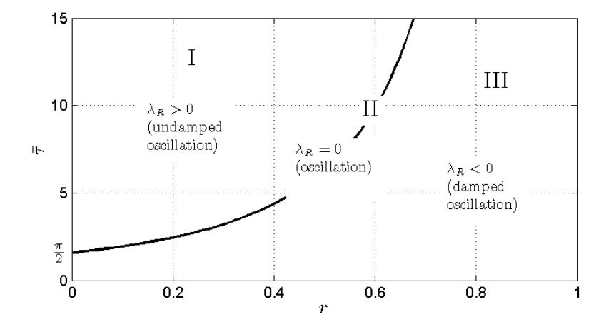
Figure 2 Bifurcation diagram for critical delay \(\overline{\tau}\) with respect to r (taken from Kasbawati, et al. [1]).
simulations are presented for three cases of the ratio \(r = G/V_1\) of the rate of glucose supply (G) and the maximum reaction rate \((V_1)\) of the first delay experienced by the enzyme (see Figure 2): r = 0.3, r = 0.4, and r = 0.5 for fixed \(\overline{\tau} = 4.4\). The parameter \(\overline{\tau} = \tau V_1/K_1\) is a critical delay for which the system generates a periodic solution in the neighborhood of steady state \(\mathbf{X}_E\) (Hopf bifurcation parameter).
To find matrix \(\mathbf{Q}_k\) in Eq. (10), an optimization procedure was constructed as follows. Let us write \(\mathbf{Q}_k = [\mathbf{q}_{ij}]\). Since \(\mathbf{J}_2\) in Eq. (2) only has two nonzero entries, then \(q_{ii}\) can be defined as follows,
\[q_{ij} = \begin{cases} p_j, & i = 1, j = 1, \dots, 7, \\ 0, & \text{otherwise,} \end{cases}\] with constants \(p_j\) that have to be determined. The objective function for the optimization problem of finding matrix \(\mathbf{Q}_k\) is defined as
\[\min_{\mathbf{p}} \left\| \mathbf{W}_{k} (\mathbf{J}_{2} \mathbf{Q}_{k}) e^{\mathbf{W}_{k} (\mathbf{J}_{2} \mathbf{Q}_{k}) + \mathbf{J}_{1}} - \mathbf{J}_{2} \right\|, \tag{17}\] where \(\|\cdot\|\) is a Euclid norm, \(\mathbf{p} = (p_1, \dots, p_7)\) are the optimization variables, \(\mathbf{W}_k(\mathbf{J}_2\mathbf{Q}_k)\) is the matrix Lambert function defined in Eq. (11), and \(\mathbf{J}_1\), \(\mathbf{J}_2\) are matrices defined in Eq. (2).
In this study, the Cuckoo Search algorithm was used to solve Eq. (17). This is a heuristic method inspired by the specific behavior of the cuckoo bird's breeding habits (see [11,12]). The computational procedures were as follows:
- 1. Set the branch of the Lambert function, number of population (nest), number of iterations, termination criteria, and probability of the eggs being detected by the host bird (in our simulations we take probability \(\beta\) equals 0.25).
- 2. Randomly generate an initial population for p using the following equation,
\[\mathbf{p}_0 = \mathbf{p}_t + \mu(\mathbf{p}_u - \mathbf{p}_t),\] where \(\mathbf{p}_l\) and \(\mathbf{p}_u\) are the lower and upper bound vector of the optimization variable \(\mathbf{p}\), respectively, and \(\mu\) is a random parameter that is generated uniformly in the interval [0,1].
- 3. Evaluate the objective function given by Eq. (17), rank the solutions, and find the current best nest.
- 4. Generate a new population using Levy flight via the Mantegna algorithm (see [11]).
- 5. Evaluate the objective function in Eq. (17) using the new population.
- 6. Apply selection using random walk and probability β to avoid the worst nests, and generate a new generation.
- 7. Return to step c), unless the termination criteria are satisfied.
The numerical results are depicted in Figures 3-5, for different values of r. In this simulation, the principal branch of the Lambert function was used as the most dominant mode. We then compared the matrix Lambert results with the Runge-Kutta results. We point out that the solutions generated from both methods were quite in agreement for all three cases of r.
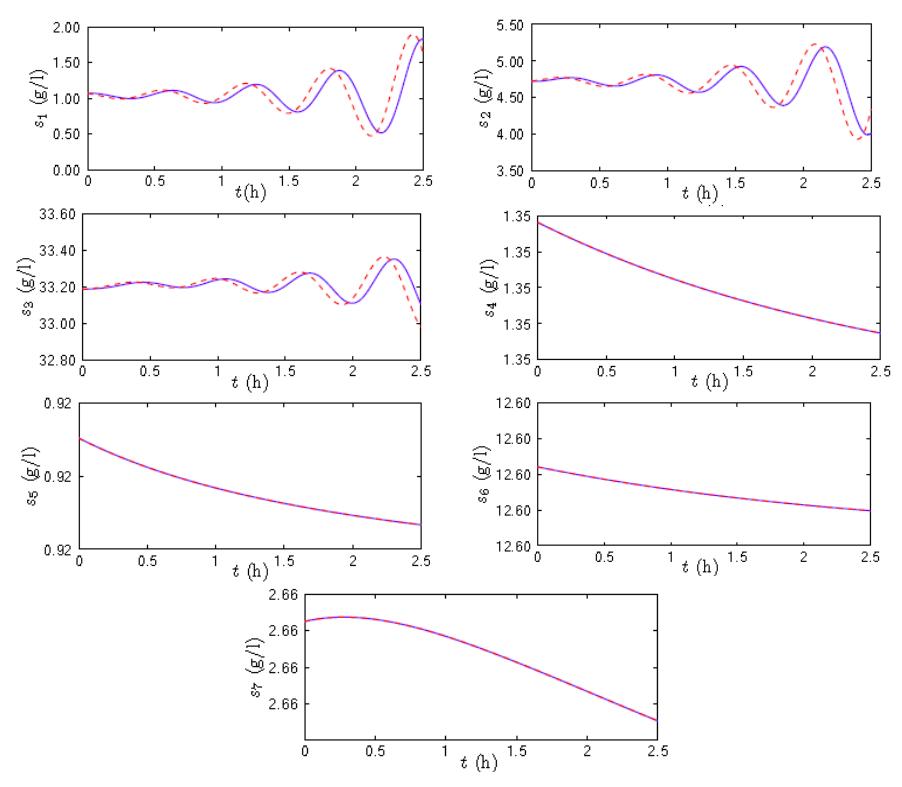
Figure 3 Comparison of Runge-Kutta solutions (dashed lines) and matrix Lambert solutions (solid lines) for r = 0.3 and τ = 4.4.
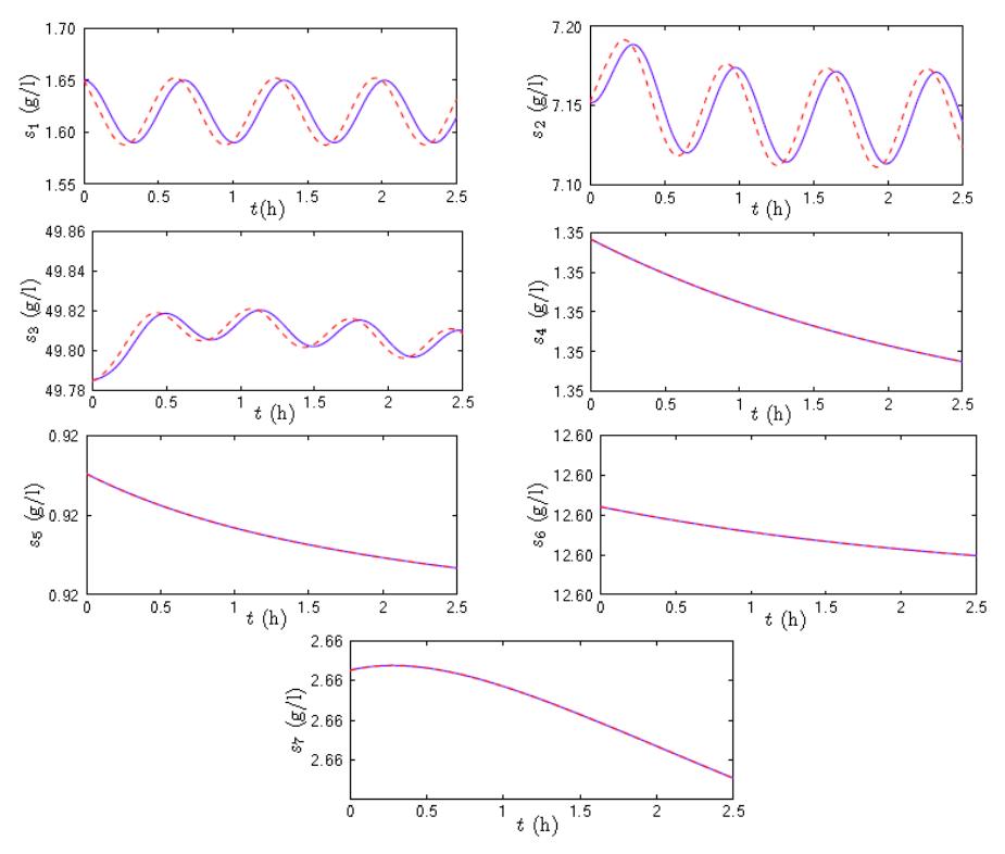
Figure 4 The comparison of Runge-Kutta solutions (dashed lines) and matrix Lambert solutions (solid lines) for r = 0.4 and \(\overline{\tau} = 4.4\).
\(\begin{tabular}{ll} \textbf{Table 2} & Eigenvalues of system given by Eq. (2) for Runge-Kutta (I) and matrix Lambert methods (II). \end{tabular}\)
| Eigenvalues of Eq. (2) for \(r = 0.3\), \(\overline{\tau} = 4.4\) | |||||||||
|---|---|---|---|---|---|---|---|---|---|
| , | \(\lambda_{_{\rm l}}\) | \(\lambda_2\) | \(\lambda_3\) | \(\lambda_4\) | \(\lambda_5\) | \(\lambda_6\) | \(\lambda_7\) | ||
| I | 0.220 + 1.690i | -2.623 | -1.083 | -0.380 | -0.251 | -0.380 | -0.380 | ||
| II | 1.550 + 2.180i | -2.623 | -1.083 | -0.380 | -0.251 | -0.380 | -0.380 | ||
| Eigenvalues of Eq. (2) for \(r = 0.4\), \(\overline{\tau} = 4.4\) | |||||||||
| \(\lambda_{l}\) | \(\lambda_2\) | \(\lambda_3\) | \(\lambda_4\) | \(\lambda_5\) | \(\lambda_6\) | \(\lambda_7\) | |||
| I | \(0.527 \times 10^{-4} - 1.570i\) | -2.571 | -1.083 | -0.380 | -0.251 | -0.380 | -0.380 | ||
| II | \(-3x10^{-4} - 9.340i\) | -2.571 | -1.083 | -0.380 | -0.251 | -0.380 | -0.380 | ||
| Eigenvalues of Eq. (2) for \(r = 0.5\), \(\overline{\tau} = 4.4\) | |||||||||
| \(\lambda_{\mathrm{l}}\) | \(\lambda_2\) | \(\lambda_3\) | \(\lambda_4\) | \(\lambda_5\) | \(\lambda_6\) | \(\lambda_7\) | |||
| I | -0.250 + 1.380i | -2.521 | -1.083 | -0.383 | -0.251 | -0.380 | -0.380 | ||
| II | -1.530 + 8.250i | -2.521 | -1.083 | -0.383 | -0.251 | -0.380 | -0.380 | ||
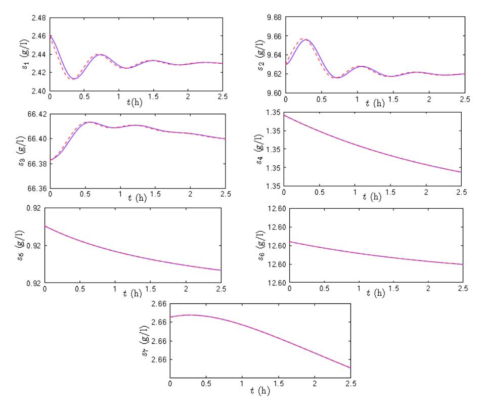
Figure 5 The comparison of Runge-Kutta solutions (dashed lines) and matrix Lambert solutions (solid lines) for r = 0.5 and \(\overline{\tau} = 4.4\).
The eigenvalues of the two methods are given in Table 2. We observe that for r = 0.3, the solutions are unstable, due to the positivity of the real part of eigenvalue \(\lambda_1\) (see Figure 3). Meanwhile, for r = 0.4, the solutions are almost periodic (see Figure 4). This is indicated by the real part of \(\lambda_i\) which is almost zero. For r = 0.5, the solutions are stable with damped oscillations (see Figure 5).
Furthermore, we quantified the mean error of the solutions generated by both methods for all three cases of r. The mean error was computed as follows:
\[e_j^{(r)} = \frac{1}{n} \sum_{i=1}^{n} \left| s_j^I(i) - s_j^{II}(i) \right|, \ j = 1, \dots, 7, \ r = 1, 2, 3,\] where n is the number of time partition, \(s_j^I(i)\) and \(s_j^{II}(i)\) are the solutions of variable j resulted from using the first and second method, respectively.
In Figure 6 we observe that for the unstable case (r=0.3), the mean error of the solutions was relatively high (see Figure 6(a)). This occurred due to the instability of the solutions. Meanwhile for the stable cases (r=0.4) and r=0.5), the mean error of the solutions was relatively small (see Figure 6(b) and (c)). This means that the present approximate method is reliable compared to the classical Runge-Kutta method, especially for the stable solutions.
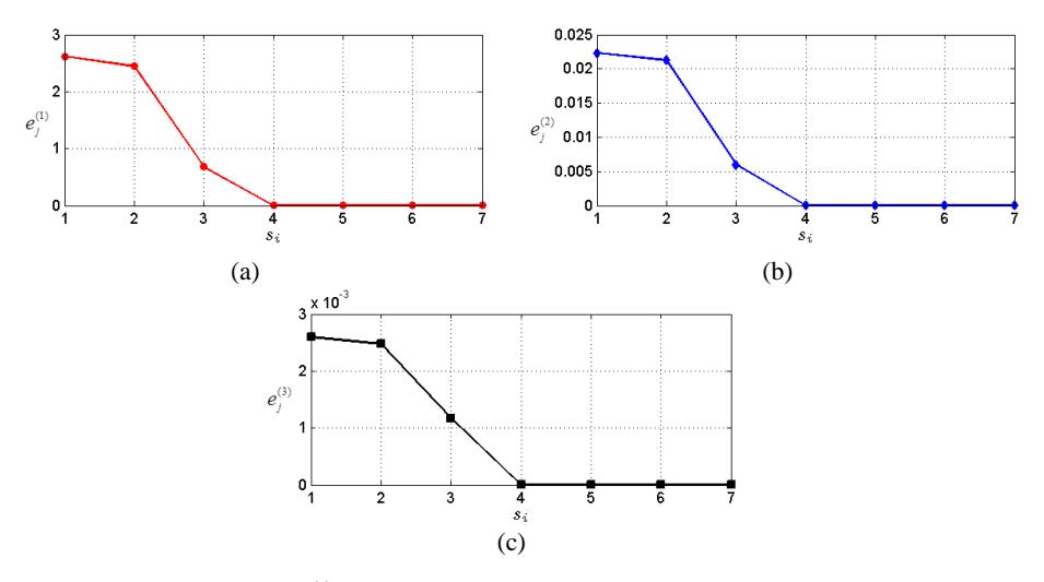
Figure 6 Mean error \(e_i^{(r)}\) of solution \(S_i\) for: (a) r = 0.3, (b) r = 0.4, (c) r = 0.5.
5 Conclusions
In this paper a different approach for generating approximate solutions of the linearized delay differential equation arising from a certain metabolic system has been presented. The closed form of the solution was generated via the matrix Lambert function written as a linear combination of the Lambert function solutions in all branches. Three dynamical behaviors of the metabolic system were presented numerically. We observed that the solutions generated via the Lambert method of the zeroth mode and the Runge-Kutta method were quite in agreement for the considered cases.
Acknowledgements
This work was partly supported by Riset KK ITB No. 213/I.1.C01/PL/2013. The second author would also like to thank DIKTI for the support received through her BPPDN scholarship.