
1 Introduction
The multifractal concept has been applied in many fields such as the study of the spatial structure of objects [1,2], turbulence [3] and geological structures [4,5]. In soil science, the multifractal concept has been applied to analyze the pore size distribution and particles of soil [6-8], the image of a thin slice of soil [9], the structure of clay [10], the matrix pore structure of a porous medium [11], soil surface pressure [12] and soil spatial variability [13]. Muller and McCauley [4] were successful in applying the fractal method to characterize the properties of the fluid flow of sedimentary rocks. Posadas, et al. [14] successfully demonstrated that multifractal parameters can quantify the spatial arrangement of soil pores so that they can be used to classify the soil structure.
In this study characteristics of the pore size distribution of peat soil were investigated. This investigation was based on image analysis and multifractal analysis. The results of both analyses were compared to obtain the relationship between physical parameters and complexity parameters.
2 Material and Method
2.1 Peat Soil Samples
The object of this study were peat soil samples taken in the area of Pontianak, West Kalimantan, precisely at the coordinates (0° 4' 2.27" S, 109°18' 48.59" E), at a depth of 30 cm from the earth surface. Samples were taken from pure peat. These samples were made in the shape of cubes, each with a size of 2 x 2 x 2 cm. The samples were dried for 7 days. The samples were reconstructed into digital data using a micro computerized tomography scanner (\(\mu\)CT scanner Skyscan 1173). Reconstruction was carried out to generate a 3D profile of the microscopic structure. Figure 1 shows a 3D projection of the sample with a volume of interest (VOI) size of 220 × 220 × 330 voxels displayed in grayscale.
Figure 1 Peat soil image in 3D with 9.41 micrometer per pixel resolution.
Information related to the physical parameters of the sample is shown in Table 1.
Tabel 1 Basic information about the sample calculated by CT Analyzer [15].
| No | Property | Value |
|---|---|---|
| 1 | Volume (mm3) | 19724 |
| 2 | Total surface(mm2) | 4387.6 |
| 3 | Thickness (mm) | 2.0508 |
| 4 | Total porosity (%) | 19.526 |
2.2 Image Processing
The 3D profile in Figure 1 was sliced into five layers. The 2D layers were considered to represent the overall structure of the peat soil. The layers were taken from the bottom to the top of the sample. Each 2D image had a size of 220 x 220 pixels (Figure 2). The images were then analyzed using multifractal methods.
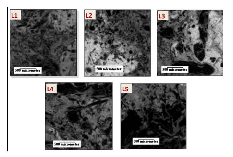
Figure 2 Peat soil gray scale image.
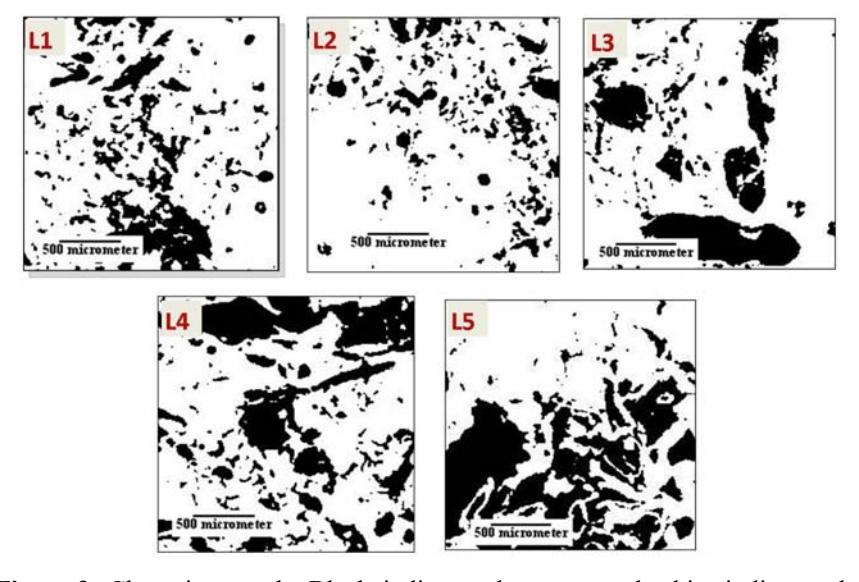
Figure 3 Clustering result. Black indicates the pores and white indicates the matrix.
The next step was that each profile in Figure 2 was thresholded using the Otsu method [16] to obtain a binary image (Figure 3). The binary image was used to distinguish between the matrix and the pores. The matrices are represented by white color and the pores are represented by black color.
The next step was calculating the parameters of the pore geometry. The calculated values of the pore geometry parameters are shown in Table 2.
| Peat Soil | Average Area | Average Diameter | Porosity | Standard Deviation | |
|---|---|---|---|---|---|
| Segment | (mm2) | (mm) | (%) | ||
| L1 | 111791.97 | 161.1 | 21.74 | 597844.08 | |
| L2 | 335428.25 | 304.0 | 13.90 | 759755.96 | |
| L3 | 160909.60 | 180.1 | 24.91 | 739793.06 | |
| L4 | 87828.65 | 190.2 | 34.42 | 657442.73 | |
| L5 | 112087.13 | 251.26 | 41.31 | 263385.45 | |
Tabel 2 Calculated pore geometry parameters of peat soil segments [17].
The peat soil segments were grouped into three categories based on average pore diameter. The first category (L1 and L2) contained slices with a low porosity (13.90-21.74%), a wide range of average pore diameter (161,1-304,0 mm) and visually random distribution. The slices from this category were taken from the bottom of the sample shown in Figure 1. The second category (L3 and L4) contained slices with intermediate porosity (24,91-34,42%) and medium average pore diameter (180,1-190,2 mm). The slices from this category were taken from the center of the sample. The third category (L5) contained slices with a large porosity (41,31%) and a small average pore diameter (140,9 mm). The slices from this group of samples were taken from the top of the sample shown in Figure 1.
2.3 Multifractal Analysis
Multifractal analysis was initiated by dividing the binary image of the peat in a \(\delta x \delta\)-sized grid, where \(\delta\) is the width of a single pixel in the grid. The next step was to calculate the density of each box \(\mu_i\). The pore density was calculated using Eq. (1) [18]:
\[\mu_i = \frac{m_i}{M} \tag{1}\] where \(m_i\) is the total number of pixels of pores in the i-th box and M is the total number of pixels in the whole.
After the pore density was obtained, the next process was to create the partition function \(\chi_q(\delta)\) by moment q (\(-\infty\) to \(+\infty\)). The partitions function of \(\mu_i(\delta)\) was calculated using Eq. (2) [19]:
\[\chi_q(\delta) = \sum_{i=1}^{n(\delta)} (\mu_i)^q \tag{2}\] where \(n(\delta)\) is the number of boxes that cover the peat soil pores when the box size is \(\delta\), and \(\mu_i\) is the density of each box.
The relationship between the partition function \(\chi_q(\delta)\) and the size of the box \(\delta\) was calculated using Eq. (3) [18]:
\[\chi_q(\delta) \propto \delta^{\tau(q)} \tag{3}\] where \(\tau(q)\) is exponential mass in the order of q, which can be obtained by plotting the data \(\chi_q(\delta)\) to \(\delta\) using a log-log plot (Figure 4).
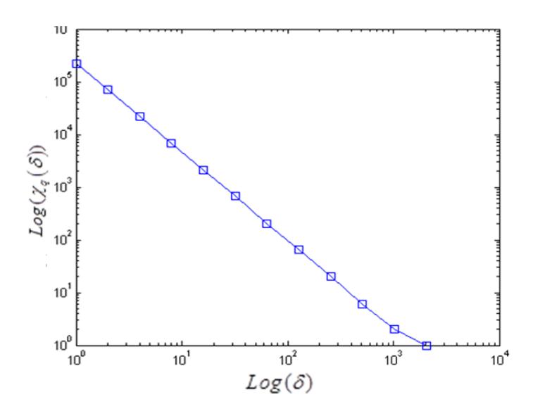
Figure 4 Example of log-log plot.
From \(\tau(q)\) and the order q, the generalized multifractal dimensions could be obtained through Eq. (4) [18]:
\[D(q) = \frac{\tau(q)}{1 - q} \tag{4}\]
The above equation is only valid if \((q \ne 1)\). If (q = 1) then multifractal dimensions can be obtained with Eq. (5) [18]:
\[D(1) = \lim_{r \to 0} \frac{\sum_{i=1}^{N(r)} \mu_i(\delta) \log \mu_i(\delta)}{\log r}\] (5)
The generalized multifractal spectrum function \(f(\alpha(q))\) was obtained through Eq. (6) [18]:
\[f(\alpha(q)) = \alpha(q)q - \tau(q) \tag{6}\] where \(\alpha(q)\) is the singularity exponent, as it describes the local degree of singularity or regularity around the point q.
If the peat soil pore distribution has multifractal behavior, then its multifractal spectrum diagram will be concave downward. Whereas if the peat soil pore distribution is monofractal, then its multifractal spectrum will be a single point.
In many cases, the multifractal property can also be described by several parameters derived from D(q) and \(\tau(q)\). On a structure that is considered to be monofractal, the value of D(q) will be the same for all values of q. A new parameter w can also be derived from D(q). This parameter is recognized as the multifractal spectrum width and can be used as an important parameter predictor. This value was obtained from Eq. (7) [20]:
\[w = D(-3) - D(3) \tag{7}\]
A greater w indicates that the spatial structure of the peat soil pores is more heterogeneous and vice versa [20].
3 Result and Discussion
The multifractal spectrum analysis results of the pore distribution for all slices of peat that were investigated are shown in Figure 5.
From Figure 5 it can be seen that all slices had a multifractal spectrum in the form of a downward concave. This means that the pore distribution of the peat had a multifractal pattern. Once it was known that the entire peat profile
behaves as a mutifractal pattern, the next step was calculating some multifractal parameters. The results for all profiles are shown in Table 3.
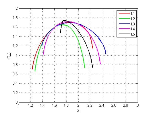
Figure 5 Multifractal spectra for the spatial distribution patterns of peat soil pores.
Posadas, et al. [14] demonstrated that the properties of f(α)-spectra can quantify and separate the spatial arrangement of contrasting soil structures. Therefore, this parameter could be used to improve the classification of the soil structures. The increasing value of max min showed that the levels of heterogeneity of the pore size distributions also increased.
Tabel 3 Multifractal parameters to characterize the spatial structure of the pores in peat soil.
| Peat Soil Segment | L1 | L2 | L3 | L4 | L5 |
|---|---|---|---|---|---|
| D(-3) | 2,00 | 1,83 | 2,12 | 2,02 | 1,91 |
| D(3) | 1,41 | 1,46 | 1,46 | 1,54 | 1,74 |
| D(0) | 1,71 | 1,65 | 1,70 | 1,72 | 1,75 |
| Δ(D(-3)-D(3)) | 0,59 | 0,37 | 0,66 | 0,48 | 0,17 |
| αmax-αmin | 1,02 | 0,84 | 1,08 | 0,96 | 0,54 |
From Table 3, it can be seen that the second group (L3 and L4) had the highest value of max min . This means that this slice category had the most heterogeneous pore size distribution. It can be seen from Figure 3 that the second category consisted of a mixture of various pore sizes. Meanwhile, the lowest value of max min was owned by the third category of peat soil slices (L5). These values confirm that the pore size distribution of this category was likely to be more homogeneous compared to the other categories. This interpretation is consistent with the direct visual observation of Figure 3 in which L5 is dominated by large-size pores.
From Figure 4 it can be seen that the first category had the most symmetric multifractal spectrum f(a). Meanwhile, the third group had the most asymmetric f(a) spectrum. A symmetric spectrum means that the structure of the peat layer is dominated by small-size pores (Figure 3). In contrast, an asymmetric spectrum means that the structure of the peat layer is dominated by large pores. The second category is in between both other states.
From Table 3, it can also be seen that changes in the average area value can be described well by changes in parameter D(0). A higher value of D(0) shows that the average area is getting smaller and vice versa.
4 Conclusion
From this study it can be concluded that the spectrum of \(f(\alpha)\) can well describe pore size distribution. It can also be concluded that the average pore size is correlated with the value of D(0). A high value of the average pore size is followed by a low D(0) value and vice versa.
Acknowledgements
This research was funded by the Directorate General of Higher Education, Ministry of Education and Culture of Indonesia, through Tanjungpura University DIPA-023.04.2.415134/2013, dated May 1<sup>st</sup>, 2013, in accordance with SPK Number 6246/UN22.13/LK/2013, dated May 10<sup>th</sup>, 2013.