
1 Introduction
Avian influenza (H5N1) is an animal disease that can be transmitted to humans through animals, such as ducks, chickens and other fowl. It is caused by influenza virus type A [1]. This virus can be classified into two groups: highly pathogenic Avian influenza A and low pathogenic Avian influenza A [2]. Avian influenza viruses have three subtypes that are able to transmit the disease to birds and humans: influenza A H5, A H9, and A H7 [2]. The symptoms when a human is infected by the Avian influenza virus are indicated by hacking, ague, coldness, and headache [3].
Avian influenza naturally occurs among poultry but infections with the virus have recently been detected among humans. The transmission of the disease to humans occurs through air contaminated with the Avian influenza virus. It originates from feces of poultry that suffers from Avian influenza. If the Avian influenza virus is transmitted to humans, it causes serious problems. In Hongkong in 1998, Avian influenza attacked humans. Sixteen cases of human infection by the virus were confirmed and three were suspected [4]. In Indonesia, humans infected by Avian influenza have been recorded in 151 cases of whom 52 died [5]. In Vietnam, similarly, 119 cases and 59 deaths have been recorder [5].
Since Avian influenza can be transmitted from poultry to humans, prevention programs to control the disease could help to reduce number of the Avian influenza cases [6]. Intervention programs and case management of Avian influenza in Indonesia have been implemented, such as maintaining cleanliness, washing hands after having contact with poultry, cleaning and spraying poultry cages with disinfectant. In addition, medical treatment and vaccination can also prevent the spread of the disease. A vaccine for poultry is available but until now a vaccine against Avian influenza for humans has not been found. Available drugs for treatment of humans infected with Avian influenza are Zanamivir and Oseltamivir.
One of the ways to prevent the spread of Avian influenza is vaccination of poultry and medical treatment of infected humans. Numerous researches have been conducted to study the behavior of Avian influenza. One of the possible approaches is through mathematical modeling. Mathematical models of Avian influenza have been developed to understand characteristics of the disease. A mathematical model that considers both spatial factors and farm volume has been developed by Manach, et al. in [7]. An ordinary differential equation model has been constructed by Iwami in [8]. Iwami's model was extended by Gumel in [9]. He developed a model of Avian influenza in which contact between human and birds (wild and domestic) is assumed and infected humans are isolated. An optimal-strategy model of Avian influenza has been built by Jung, et al. [10]. In [11], Vaidya, et al. studied the dynamics of the Avian influenza virus in wild birds. Martcheva built a model of Avian influenza in [12] that combines models of humans suffering from influenza.
The present study modeled the pattern of Avian influenza spread with vaccination and medical treatment. The basic reproduction ratio (R0) was determined as well as the existence point of endemic and non-endemic equilibrium. Furthermore, the model of the vaccination and medical treatment schedules can be used to provide vaccination and medical treatment strategies. A genetic algorithm is used to find the optimal solutions of the objective function.
2 Mathematical Model
The mathematical model of the Avian influenza in humans and poultry was constructed based on the following assumptions. First, the birth rate of the humans is constant, the birth rate of the poultry is not constant. Second, the poultry population lives in a livestock area. Third, Avian influenza causes death in poultry and humans. Fourth, transmission of Avian influenza occurs from poultry to humans but it is not transmitted from humans to poultry. Fifth, vaccinations are given to susceptible poultry and medical treatment are given to infected humans. Sixth, humans and poultry are born in a susceptible state. Seventh, infected poultry having contact with humans and other poultry results in infection. Lastly, medical treatment is given periodically.
The mathematical model is based on the transmission diagram shown in Figure 1. Table 1 shows the variables and parameters. The mathematical model of Avian influenza in human and poultry populations is given in Eq. (1).
Table 1 Variables and parameters.
| Symbol | Parameter Definition | Dimension | |
|---|---|---|---|
| Sh(t) | Number of susceptible humans | Human | |
| Ih(t) | Number of infected humans | Human | |
| Rh(t) | Number of recovered humans | Human | |
| T(t) | Number of treated humans | Human | |
| Sv(t) | Number of susceptible poultry | Poultry | |
| Iv(t) | Number of infected poultry | Poultry | |
| V(t) | Number of vaccinated poultry | Poultry | |
| A | Human recruitment rate | Human/Time | |
| Av | Poultry recruitment rate | Poultry/Time | |
| bh | Successful transmission rate for poultry to human | 1/Time | |
| bv | Successful transmission rate for poultry to poultry | 1/Time | |
| | Transition rate of humans from treated humans to susceptible humans | 1/Time | |
| | Transition rate of humans from recovered humans to susceptible humans | 1/Time | |
| | Transition rate of humans from infected humans to susceptible humans | 1/Time | |
| µ | Natural death rate of humans | 1/Time | |
| Ө | Harvest rate of poultry population | 1/Time | |
| | Virulence of humans | 1/Time | |
| δv | Virulence of poultry | 1/Time | |
| | Rate of treatment of infected humans | 1/Time | |
| | Rate of vaccination of susceptible poultry | 1/Time | |
| | Recovery rate due to treatment | - | |
| h | Cost function of treatment of infected humans | 1/human | |
| v | Cost function of vaccination of susceptible poultry | 1/poultry | |
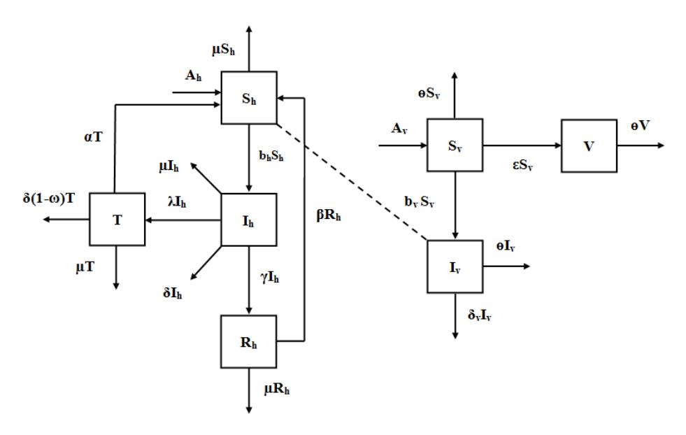
Figure 1 Transmission diagram of Avian influenza in humans and poultry.
\[\frac{dS_{v}}{dt} = A_{v} - \left(\frac{b_{v}I_{v}}{S_{v} + I_{v} + V} + \theta + \varepsilon\right)S_{v}\] \[\frac{dI_{v}}{dt} = \frac{b_{v}I_{v}}{S_{v} + I_{v} + V}S_{v} - (\theta + \delta_{v})I_{v}\] \[\frac{dV}{dt} = \varepsilon S_{v} - \theta V\] \[\frac{dS_{h}}{dt} = A - \left(\frac{b_{h}I_{v}}{S_{v} + I_{v} + V} + \mu\right)S_{h} + \beta R_{h}\] \[\frac{dI_{h}}{dt} = \frac{b_{h}I_{v}}{S_{v} + I_{v} + V}S_{h} - (\mu + \gamma + \delta + \lambda)I_{h}\] \[\frac{dR_{h}}{dt} = \gamma I_{h} - (\mu + \beta)R_{h} + \alpha T\] \[\frac{dT}{dt} = \lambda I_{h} - \delta(1 - \omega)T - \mu T - \alpha T\] (1)
2.1 Analysis of the Model
2.1.1 Equilibrium Point
Here, we are trying to figure out the equilibrium points in the area that is denoted by \(\Omega\), as follows:
\[\Omega = \{(S_v, I_v, V, S_h, I_h, R_h, T) \in \mathfrak{R}_+^7\}.\]
The model has two possible equilibria: the disease-free equilibrium and the endemic equilibrium. The disease free equilibrium of the model for poultry is
\[E_0 = (S_v, 0, V, S_h, 0, 0, 0)\] with \(S_v = \frac{A_v}{\theta + \varepsilon}\), \(V = \frac{\varepsilon A_v}{\theta(\theta + \varepsilon)}\), and \(S_h = \frac{A}{\mu}\).
Define, \[R_1 = \frac{b_V \theta}{(\theta + \varepsilon)(\theta + \delta_V)}\].
The endemic equilibrium of the Avian influenza model of poultry is \(E_1 = (S_v, I_v, V, S_h, I_h, R_h, T)\) with
\[\begin{split} S_{v} &= \frac{(\theta + \delta_{v})A_{v}R_{1}}{(R_{1} - 1)\delta_{v}b_{v} + \theta b_{v}R_{1}} \,, \\ I_{v} &= \frac{(R_{1} - 1)b_{v}S_{v}}{(\delta_{v} + \theta)R_{1}} \,, \\ V &= \frac{\varepsilon A_{v}}{(\theta + \varepsilon)(\theta R_{1} + \delta_{v}(R_{1} - 1))} \,, \\ S_{h} &= \frac{AR_{1}(\mu + \beta)(\mu(1 - \omega)\delta + \alpha)(\mu + \lambda + \gamma + \delta)}{(R_{1} - 1)B_{1} + R_{1}B_{2}} \,, \\ I_{h} &= \frac{(\mu + \beta)(\mu(1 - \omega)\delta + \alpha)bA}{(R_{1} - 1)(B_{1} + R_{1}B_{2})} \,, \\ R_{h} &= \frac{Ab(R_{1} - 1)((\gamma(1 - \omega)\delta + \alpha + \mu) + \lambda\alpha)}{(R_{1} - 1)B_{1} + R_{1}B_{2}} \,, \\ T &= \frac{Ab(R_{1} - 1)\lambda(\mu + \beta)}{(R_{1} - 1)B_{1} + R_{1}B_{2}} \,. \end{split}\]
Where
\[\begin{split} B_1 &= b\beta((1-\omega)\delta(\delta+\lambda+\mu) + \mu(\mu+\alpha+\lambda+2\delta)) + b\mu((1-\omega)\delta+\mu+\alpha)(\mu+\delta+\gamma+\lambda)\mathbb{Z} \\ B_2 &= (1-\omega)\delta + \mu + \alpha)\mu(\mu+\beta)(\mu+\delta+\gamma+\lambda). \end{split}\]
The endemic equilibrium \(E_1\) exists if and only if \(R_1 > 1\).
Theorem 1. The Avian influenza model has \(E_0 = (S_v, 0, V, S_h, 0, 0, 0)\) as the non-endemic equilibrium point. It is locally asymptotically stable if and only if \(R_1 > 1\).
Proof. We study the stability of \(E_0 = (S_v, 0, V, S_h, 0, 0, 0)\). The corresponding Jacobian matrix \(D_{E_n}\) is as follows
\[J_{E_0} = \begin{bmatrix} -(\theta + \varepsilon) & -\frac{b_v \theta}{\theta + \varepsilon} & 0 & 0 & 0 & 0 & 0 & 0 \\ 0 & \frac{b_v \theta}{\theta + \varepsilon} - (\theta + \delta_v) & 0 & 0 & 0 & 0 & 0 \\ \varepsilon & 0 & -\theta & 0 & 0 & 0 & 0 & 0 \\ 0 & -\frac{bA\theta}{A_v \mu} & 0 & -\mu & 0 & \beta & 0 \\ 0 & \frac{bA\theta}{A_v \mu} & 0 & 0 & -(\mu + \lambda + \delta + \gamma) & 0 & 0 & 0 \\ 0 & 0 & 0 & 0 & \gamma & -(\mu + \beta) & \alpha \\ 0 & 0 & 0 & 0 & 0 & \lambda & 0 & -(\delta(1 - \omega) + \mu + \alpha) \end{bmatrix}.\]
Eigenvalues of \(J_{E_0}\) are
\[\begin{split} x_1 &= -\theta \,, \\ x_2 &= -(\theta + \varepsilon) \,, \\ x_3 &= -\mu \,, \\ x_4 &= -(\mu + \beta) \,, \\ x_5 &= -((1 - \omega)\delta + \mu + \alpha) \,, \\ x_6 &= (R_1 - 1)(\theta + \delta_v) \,, \\ x_7 &= -(\mu + \delta + \lambda + \gamma) \,. \end{split}\]
Observe that \(a_1, b_1, c_1\) when \(R_1 > 1\). Therefore all of the eigenvalues of \(J_{E_0}\) are negative if and only if \(R_1 < 1\). This proves Theorem 1.
Theorem 2. The Avian influenza model has \(E_1 = (S_v, I_v, V, S_h, I_h, R_h, T)\) as the endemic equilibrium point. It is locally asymptotically stable if and only if \(R_1 > 1\).
Proof. We study the stability of \(E_1 = (S_v, I_v, V, S_h, I_h, R_h, T)\). The corresponding Jacobian matrix \(D_{E_0}\) is as follows
\[J_{E_1} = \begin{bmatrix} D_1 & 0 \\ D_3 & D_4 \end{bmatrix},\] where
\[D_{1} = \begin{bmatrix} \frac{b_{v}I_{v}S_{v}}{(S_{v} + I_{v} + V)^{2}} - \frac{b_{v}I_{v}S_{v}}{S_{v} + I_{v} + V} - (\theta + \varepsilon) & -\frac{b_{v}S_{v}}{S_{v} + I_{v} + V} + \frac{b_{v}I_{v}S_{v}}{(S_{v} + I_{v} + V)^{2}} & \frac{b_{v}I_{v}S_{v}}{(S_{v} + I_{v} + V)^{2}} \\ -\frac{b_{v}I_{v}S_{v}}{(S_{v} + I_{v} + V)^{2}} + \frac{b_{v}I_{v}S_{v}}{S_{v} + I_{v} + V} & \frac{b_{v}S_{v}}{S_{v} + I_{v} + V} - \frac{b_{v}I_{v}S_{v}}{(S_{v} + I_{v} + V)^{2}} - (\theta + \delta_{v}) & -\frac{b_{v}I_{v}S_{v}}{(S_{v} + I_{v} + V)^{2}} \\ \varepsilon & 0 & \theta \end{bmatrix}\] and
\[D_4 = \begin{bmatrix} -\frac{bI_v}{S_v + I_v + V} - \mu & 0 & \beta & 0 \\ \frac{bI_v}{S_v + I_v + V} & -(\mu + \lambda + \delta + \gamma) & 0 & 0 \\ 0 & \gamma & -(\mu + \beta) & \alpha \\ 0 & \lambda & 0 & -(\delta(1 - \omega) + \mu + \alpha) \end{bmatrix}.\]
The eigenvalues of \(J_{E_1}\) are given by the eigenvalues of \(D_1\) and \(D_4\). The characteristic polynomial of the matrix \(D_1\) is \(p(x) = x^3 + a_2 x^2 + a_1 x + a_0\), where
\[a_2 = \theta(R_1 + 1) + \delta_{\nu}(R_1 - 1) + \frac{\delta_{\nu} \varepsilon}{\theta}(R_1 - 1) + \varepsilon R_1,\]
\[a_{1} = (R_{1} - 1) \left( 3\delta_{v}\varepsilon + 3\delta_{v}\theta + \varepsilon\theta + \delta_{v}^{2} + \frac{\delta_{v}^{2}\varepsilon}{\theta} + \theta \right) + R_{1}\left(\theta + \varepsilon\right) - \frac{(R_{1} - 1)}{R_{1}}\left(\delta_{v}^{2} + \delta_{v}\theta\right),\] \[a_{0} = \frac{(R_{1} - 1)R_{1}b_{v}^{2}\theta^{2}(2\delta_{v} + \theta)}{R_{1}^{2}}.\]
Observe that \(a_2\), \(a_1\), \(a_0 > 1\) when \(R_1 > 1\). Therefore, the roots of the characteristic polynomial p(x) are negative if \(R_1 > 1\). The characteristic polynomial of the matrix \(D_4\) is \(q(x) = x^4 + b_3 x^3 + b_2 x^2 + b_1 x + b_0\), where
\[\text{[rumus tidak dapat ditampilkan dengan baik — lihat PDF asli]}\]
Observe that \(a_3, a_2, a_1, a_0 > 0\) when \(R_1 > 1\). Therefore, the roots of the characteristic polynomial q(x) are negative if \(R_1 > 1\). We deduce that \(E_1\) is locally asymptotically stable when \(R_1 > 1\). This proves Theorem 2.
2.1.2 Basic Reproduction Ratio
The basic reproduction ratio is an important parameter in the epidemiology of infectious diseases. It is defined as the expected number of secondary cases rising from one infected person who encounters a closed susceptible population [13]. The notation that is often used for this parameter is \(R_0\). It can be obtained in several ways. In this study, \(R_0\) was obtained by building a matrix that generates a number of new infected individuals. This matrix is usually denoted by K and called Next-Generation Matrix (NGM). NGM is evaluated at the value of the non-endemic equilibrium point, which is obtained by
\[K = \begin{bmatrix} \frac{b_v \theta}{(\theta + \varepsilon)(\theta + \delta_v)} & 0\\ \frac{bA\theta}{A_v \mu(\theta + \delta_v)} & 0 \end{bmatrix}.\]
The largest eigenvalue of K is
\[R_0 = \frac{b_{\mathcal{V}}\theta}{(\theta + \varepsilon)(\theta + \delta_{\mathcal{V}})}.\]
We know that \(R_0\) is equal to \(R_1\) as defined in the equilibrium point subsection. The vaccination parameter (\(\epsilon\)) affects the value of \(R_0\). If the Avian influenza is endemic in poultry, the virus will be endemic in humans. The parameters that can be controlled to prevent endemic Avian influenza are vaccination and the harvesting of the poultry.
3 Optimization Model
An optimal vaccination strategy in a deterministic model was introduced by Hethcote and Waltman in [14]. They developed the model to optimize the vaccination schedule in an epidemic model. In the present study, the optimization model describes a vaccination and medical treatment scenario within a certain period to reduce the number of Avian Influenza cases. Therefore, there are two control parameters to be considered: the rate of medical treatment for infected humans (\(\lambda\)) and the rate of vaccination for susceptible poultry (\(\epsilon\)).
If the rate of vaccination and medical treatment increases, then the total costs required to manage the disease also increase. Vaccination and medical treatment costs are influenced by many other factors, such as labor costs, operational costs, etc. Therefore, the following objective function was used:
\[\begin{aligned} \text{Minimize } f &= \omega_h \left( \int\limits_0^{\Delta t_1} I_{h\lambda_1}(t) dt + \int\limits_{\Delta t_1}^{\Delta t_2} I_{h\lambda_2}(t) dt + \ldots + \int\limits_{\Delta t_{n-1}}^{\Delta t_n} I_{h\lambda_2}(t) dt \right) + \\ & \omega_v \left( \int\limits_0^{\Delta t_1} S_{v\varepsilon_1}(t) dt + \int\limits_{\Delta t_1}^{\Delta t_2} S_{v\varepsilon_2}(t) dt + \ldots + \int\limits_{\Delta t_{n-1}}^{\Delta t_n} S_{v\varepsilon_2}(t) dt \right), \end{aligned}\] (2)
where \(t \in \Re\), k is the number of times to deliver the medicine and vaccine at time t or \(k = \frac{T_m}{\Delta}\), \(\Delta\) is the duration of the period during which to deliver the medicine and vaccine, \(\lambda_j\) and \(\mathcal{E}_j\) are the rates of medical treatment and vaccination, \(\psi_h\) and \(\psi_v\) are the cost functions, \(I_{h\lambda_j}\) is the number of infected humans who are given medical treatment at the \(j^{th}\) period, and \(S_{v\mathcal{E}_j}\) is susceptible poultry that is given vaccine at the \(j^{th}\) period, j = 1, 2, 3, ..., n. The objective function in Eq. (2) has the following constraint:
\[I_{h}(t) + R_{h}(t) + T(t) \le A,\] \[\max_{(0,t)} I_{h}(t) \le B,\] \[\max_{(0,t)} I_{v}(t) \le C.\] (3)
Here A, B and C are the maximum numbers of Avian influenza cases. The mathematical problem to be solved is to minimize Eq. (2) with the constraint in Eq. (3) satisfying Eq. (1). This problem is solved by a genetic algorithm.
4 Numerical Simulation
This section illustrates the dynamics of an infected human compartment and scenarios for controlling Avian influenza. The simulation was done using a genetic algorithm. The values of the parameters and the initial conditions are given in Table 2. The simulated time period was divided into six periods. For each period, the initial conditions were obtained from the results of the ending point of the previous period of simulation. The objective function was calculated from the integral of susceptible poultry and infected humans multiplied by the cost function.
The results of the simulation are shown in Table 3 and Figure 2. Table 3 shows the minimum of the objective function for control of the Avian influenza with the vaccination and medicine treatment scenario. The total period of time for vaccination and medical treatment was two years divided into six periods. For each period, we administered the proper rate of vaccination and medical
treatment. Based on these results we can apply design scenarios for preventing Avian influenza infection. For example, during the first period, vaccination was given to susceptible poultry at a rate of 0.319 per time and medical treatment was given to infected humans at a rate of 0.748 per time. The vaccination rates and the medical treatment for the following period were as shown in Table 3. Therefore, we obtained a cost of 22,398,171 cost units.
Table 2 Initial condition and parameter values.
| Symbol | Value |
|---|---|
| Sh(t) | 900 human |
| Ih(t) | 5 human |
| Rh(t) | 0 |
| T(t) | 0 |
| Sv(t) | 300 poultry |
| Iv(t) | 100 poultry |
| V(t) | 0 |
| t | [0, 24] |
| | 0.00128 month-1 |
| v | 0.0208 month-1 |
| h b | 0.5 month-1 |
| b v | 0.7 month-1 |
| | 0.7 month-1 |
| | 0.0417 month-1 |
| | 0.03 month-1 |
| | 0.3 month-1 |
| v | 0.6 month-1 |
| | 0.1 |
| | 4 |
| h | 10,000 human-1 |
| v | 15,000 poultry-1 |
| A | 120 human |
| B | 100 human |
| C | 150 poultry |
The dynamics of infected humans are illustrated in Figure 2. In this figure, four simulated cases are shown, i.e. the infected human population without medical treatment or vaccination; only medical treatment; only vaccination; with medical treatment and vaccination.
Using the scenarios in Table 2, the number of Avian influenza cases were reduced 36.26% with vaccination and medical treatment, 25.68% with vaccination only, and 24.72% with medical treatment only. If the budget is limited, medical treatment is more effective than only vaccination for a short period. Over a longer period, however, the poultry vaccination scenario significantly reduces the number of the infected humans. The best result in this simulation was reached when both medical treatment and vaccination were given to the host and vector population.
| Table 3 Optimization results | ١. |
|---|
| Period | λ | ε | \[\int\limits_{\Delta t_i}^{\Delta t_{i+1}} I_{h\lambda_{i+1}} dt\] | \[\int\limits_{\Delta t_{i}}^{\Delta t_{i+1}} s_{v\varepsilon_{i+1}} dt\] | Objective function |
|---|---|---|---|---|---|
| 0-4 | 0.748 | 0.319 | 820.116 | 145.099 | |
| 4-8 | 0.795 | 0.449 | 138.175 | 81.144 | |
| 8-12 | 0.585 | 0.546 | 733.676 | 12.447 | 22,398,171 |
| 12-16 | 0.637 | 0.541 | 63.559 | 1.556 | |
| 16-20 | 0.709 | 0.502 | 65.605 | 0.145 | |
| 20-24 | 0.608 | 0.635 | 58.079 | 0.014 |
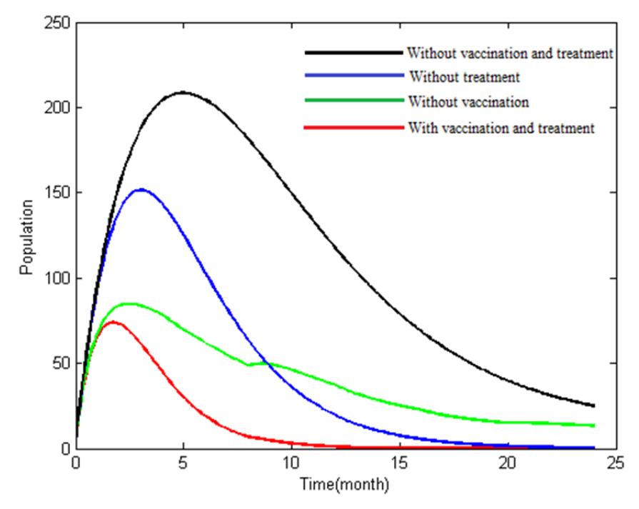
Figure 2 Numerical simulation of infected humans.
5 Conclusions
A model of Avian influenza with vaccination and medical treatment was developed in this study. The model illustrates the dynamics of Avian influenza transmission. In it, the human population is divided into four compartements: susceptible, infected, recovered, and treated. Meanwhile, the poultry population is divided into three compartments: susceptible, infected and vaccinated. The basic reproduction ratio and equilibrium points, i.e. the disease-free and the endemic equilibrium of the model, were obtained along with the basic reproduction ratio (R0) for the poultry. It was shown that endemic Avian influenza in poultry will cause endemic Avian influenza in humans. The diseasefree equilibrium was locally asymptotically stable when R0 < 1 and the endemic equilibrium was locally asymptotically stable when R0 > 1. Prevention of endemic Avian influenza can be achieved by vaccination of the poultry and medical treatment of infected humans. Optimization to reduce the number of cases of human Avian influenza infection were presented in this paper. Numerical simulation of the optimization model indicated that the dynamics of human infection decreases significantly when the Avian influenza virus is controlled by vaccination and medical treatment. In addition, the optimum vaccination and medical treatment schedules were also determined, indicating a strategy for controlling the disease over any certain period of time.
Acknowledgement
This research was founded by Riset Kelompok Keahlian ITB.