
1 Introduction
Pearson's correlation coefficient [1] is one of the most often used methods to estimate the correlation coefficient (ρ) between two random variables (X and Y) for a bivariate normality assumption of the data [2-3]. In some problems, we may have data with outliers that may arise for purely deterministic reasons: a reading, recording, or calculating error in the data [4]. In this case, using Pearson's correlation coefficient may not be suitable for the estimation of ρ because it is based on the sample means of random variables X and Y, which are known to be very sensitive to the presence of outliers [5-8]. Consequently, many robust estimators of ρ are proposed based on different underlying methodologies to resist outliers in data. For example, two well-known, nonparametric correlation coefficients are Spearman's rho and Kendall's tau correlation coefficients [9-11], which are based on the ranks of the observations. These correlation coefficients are measurements of association between two variables that are measured in at least an ordinal scale [11]. However, Abdullah [5] suggests that these correlation coefficients are not sufficiently robust estimators when the percentage of outliers in the data increases. Moreover, Evandt, et al. [12] recommends that Kendall's tau correlation coefficient is heavily biased for most values of ρ. Genest and Plante [13] have proposed
Plantagenet's correlation coefficient, which is the rank correlation measure for outlier weight and is a symmetric version of Blest's correlation coefficient [14]. Maturi and Elsayigh [2] studied the efficiency of Plantagenet's correlation coefficient and found that it has the lowest standard error compared with other weighted correlation coefficients when the data are contaminated with outliers. In this paper, the composite correlation coefficient of two random variables is proposed. This rank correlation coefficient is based on a symmetrized version of Blest's index and the jackknife procedure [15-16] is applied for bias reduction as in the studies of Balakrishnan and Tony Ng [17], Smith and Pontius [18] and Sinsomboonthong [19]. Furthermore, a simulation study was undertaken to compare the robustness with regard to data with outliers of the four estimators: the composite, Spearman's rho, Kendall's tau and Plantagenet's correlation coefficients.
2 Materials and Methods
2.1 Rank Correlation Measures
In the parametric case, the usual measure of correlation is Pearson's correlation coefficient. This estimator requires variables that represent measurement in at least an interval scale and assume that the observations are sampled from a bivariate normal distribution [11]. If the assumptions associated with this estimator are unrealistic, then nonparametric correlation coefficients, which are presented in this section, may be used. Let \((x_1, y_1),...,(x_n, y_n)\) be n observations from a population that require that both variables X and Y are measured in at least an ordinal scale. Four measures of the degree of association or correlation between the two sets of ranks are studied as follows:
2.1.1 Spearman's Rho Correlation Coefficient
A familiar nonparametric correlation coefficient [11] is Spearman's rho correlation coefficient, \(r_s\), which is given by \(r_S = 1 - \frac{6D_S^2}{n(n^2-1)}\), where \(D_S^2 = \sum_{i=1}^n (p_i - q_i)^2\), \(p_i\) and \(q_i\) are the ranks of the \(x_i\) and \(y_i\), respectively.
2.1.2 Kendall's Tau Correlation Coefficient
Kendall's tau correlation coefficient, \(r_K\), is one of the nonparametric correlation coefficients [11] and is defined by \(r_K = \frac{2K}{n(n-1)}\) and K = C - D, where C is the number of concordant pairs and D is the number of discordant pairs. A concordant pairs occurs when the rank of the second variable is greater than the rank of the former variables. A discordant pair occurs when the rank of the second variable is equal to or less than the rank of the former variables.
2.1.3 Plantagenet's Correlation Coefficient
Genest and Plante [13] proposed Plantagenet's correlation coefficient, \(r_{PG}\), which is given by \(r_{PG} = -\frac{4n+5}{n-1} + \frac{6}{n^3-n} \sum_{i=1}^n p_i q_i \left(4 - \frac{p_i + q_i}{n+1}\right)\), where \(p_i\) and \(q_i\) are the ranks of the \(x_i\) and \(y_i\), respectively.
2.1.4 Proposed Rank Correlation Coefficient
Scarsini [20] introduced a set of axioms for concordance measures of ordered pairs of continuous random variables. Let \(Q: \Upsilon(\Omega) \times \Upsilon(\Omega) \to \mathbb{R}\) be the function that satisfies the symmetry axiom, which is \(Q(x_i, y_i) = Q(y_i, x_i)\), where \(\Upsilon(\Omega)\) is a set of all real-valued continuous random variables on some probability apace \((\Omega, \mathcal{A}, \mathcal{P})\). A composite correlation coefficient, \(r_C\), is proposed to estimate the correlation coefficient between the two sets of ranks. Initially, the proposed estimator was derived based on Blest's correlation coefficient [14], \(r_B\), which is given by Eq. (1).
\[r_B = \frac{2n+1}{n-1} - \frac{12}{n(n+1)^2(n-1)} \sum_{i=1}^n (n+1-p_i)^2 q_i\] (1)
where \(p_i\) and \(q_i\) are the ranks of the \(x_i\) and \(y_i\), respectively. Genest and Plante [13] suggested the adapted Blest's correlation coefficient, \(r_{AB}\), which is given by Eq. (2), in order to meet the requirements of Scarsini's symmetry [20].
\[r_{AB} = \frac{2n+1}{n-1} - \frac{12}{n(n+1)^2(n-1)} \sum_{i=1}^{n} (n+1-q_i)^2 p_i\] (2)
Therefore, \(r_B = Q(x_i, y_i)\) and \(r_{AB} = Q(y_i, x_i)\) meet the symmetry property, which states that \(r_B\) and \(r_{AB}\) are equivalent values. This conforms to the Scarsini [20] as mentioned above. We propose a composite correlation coefficient that is derived based on \(r_B\) and \(r_{AB}\) as shown in Proposition 2.1.
Proposition 2.1 Let \((x_1, y_1),...,(x_n, y_n)\) be n observations for a sample from a population that require that both variables X and Y are measured in at least an ordinal scale. Let \(p_i\) and \(q_i\) denote the ranks of \(x_i\) and \(y_i\) among the x and y data, respectively. It is assumed there are no tied ranks. Let \(r_B\) and \(r_{AB}\) be the two rank correlation coefficients given by Eqs. (1) and (2), respectively. The composite correlation coefficient, \(r_C\), is given by Eq. (3).
\[r_{C} = n\hat{\delta} - \frac{(n-1)}{n} \sum_{i=1}^{n} \hat{\delta}_{(-i)}\] (3)
where \(\hat{\delta}\) and \(\hat{\delta}_{(-i)}\) are defined as the formulas of Eqs. (4) and (5), respectively.
\[\hat{\delta} = \frac{2n+1}{n-1} - \frac{6}{n(n+1)^2(n-1)} \sum_{i=1}^n \left[ (n+1-p_i)^2 q_i + (n+1-q_i)^2 p_i \right]\] (4)
\[\hat{\delta}_{(-i)} = \frac{2n-1}{n-2} - \frac{6}{(n-1)n^2(n-2)} \sum_{j\neq i}^{n} \left[ (n-p_{ij})^2 q_{ij} + (n-q_{ij})^2 p_{ij} \right]\] (5)
\(p_{ij}\) and \(q_{ij}\) are the ranks of \(x_j\) and \(y_j\), respectively, of the i<sup>th</sup> jackknife sample \(S_{(-i)}\) for i = 1, 2, ..., n.
Proof. Let \(r_B\) and \(r_{AB}\) be the Blest's and adapted Blest's correlation coefficients. It is assumed the weights of \(r_B\) and \(r_{AB}\) are such that \(w_B=w_{AB}=1/2\). The estimator of the rank correlation coefficient between the two sets of ranks is denoted by \(\hat{\delta}\), which is the combination of these two correlation coefficients and written as Eq. (6).
\[\hat{\delta} = w_B r_B + w_{AB} r_{AB}\] \[= \frac{2n+1}{n-1} - \frac{12}{n(n+1)^2 (n-1)} \left( \frac{1}{2} \sum_{i=1}^n (n+1-p_i)^2 q_i + \frac{1}{2} \sum_{i=1}^n (n+1-q_i)^2 p_i \right)\] \[= \frac{2n+1}{n-1} - \frac{6}{n(n+1)^2 (n-1)} \sum_{i=1}^n \left[ (n+1-p_i)^2 q_i + (n+1-q_i)^2 p_i \right]\](6)
\(\hat{\delta}\) is derived from a combination of two estimators by using a half of them. This is the empirical rank correlation coefficient as studied by Genest and Plante [13].
Let \(S_{(-i)} = \{(x_1, y_1), (x_2, y_2), ..., (x_{i-1}, y_{i-1}), (x_{i+1}, y_{i+1}), ..., (x_n, y_n)\}\) be the i<sup>th</sup> jackknife sample, which consists of the data with the i<sup>th</sup> observation removed, \(p_{ij}\) denote the rank of \(x_j\) among the x data of the i<sup>th</sup> jackknife sample \(S_{(-i)}\) and similarly \(q_{ij}\) denote the rank of \(y_j\) among the y data of the i<sup>th</sup> jackknife sample \(S_{(-i)}\) for i = 1, 2, ..., n. By using the i<sup>th</sup> jackknife sample, the estimator of correlation that corresponds to \(\hat{\delta}\) can be computed with Eq. (7).
\[\hat{\delta}_{(-i)} = \frac{2(n-1)+1}{(n-1)-1} - \frac{6\sum_{j\neq i}^{n} \left[ \left\{ (n-1)+1-p_{ij} \right\}^{2} q_{ij} + \left\{ (n-1)+1-q_{ij} \right\}^{2} p_{ij} \right]}{(n-1)\left\{ (n-1)+1 \right\}^{2} \left\{ (n-1)-1 \right\}}\] \[= \frac{2n-1}{n-2} - \frac{6}{(n-1)n^{2}(n-2)} \sum_{j\neq i}^{n} \left[ \left( n-p_{ij} \right)^{2} q_{ij} + \left( n-q_{ij} \right)^{2} p_{ij} \right]\](7)
The composite correlation coefficient, \(r_C\), is proposed in the form of an average of pseudo jackknife values as given by Eq. (8).
\[r_{C} = \frac{1}{n} \sum_{i=1}^{n} \left[ n\hat{\delta} - (n-1)\hat{\delta}_{(-i)} \right] = \frac{1}{n} \left[ n^{2}\hat{\delta} - (n-1) \sum_{i=1}^{n} \hat{\delta}_{(-i)} \right]\] \[= n\hat{\delta} - \frac{(n-1)}{n} \sum_{i=1}^{n} \hat{\delta}_{(-i)}\] (8)
where \(\hat{\delta}\) and \(\hat{\delta}_{(-i)}\) are defined as the formulas of Eqs. (6) and (7), respectively.
2.2 Properties of Point Estimator
In this section, two properties of the point estimator in terms of absolute bias and mean square error are defined to help decide whether one estimator is better than the other [21].
Definition 2.1 Let \(\hat{\theta}\) be an estimator of \(\theta\). \(ABS(\hat{\theta}) = |E(\hat{\theta}) - \theta|\) is defined to be the absolute bias of \(\hat{\theta}\). The mean square error of \(\hat{\theta}\) is defined as \(MSE(\hat{\theta}) = E(\hat{\theta} - \theta)^2\).
\(ABS(\hat{\theta})\) can be either positive or zero. \(\hat{\theta}\) is called an unbiased estimator if \(ABS(\hat{\theta}) = 0\). Otherwise, it is said to be biased. We generally prefer an estimator with a small mean square error.
3 Results of a Simulation Study
In the numerical study, we generated examples of the data from a bivariate normal distribution. A simulation study was conducted using 228 situations in order to compare the robustness properties of the proposed estimator, \(r_C\), with the three estimators (\(r_S\), \(r_K\) and \(r_{PG}\)) when the data were contaminated with outliers. In the study, samples (x,y) of four sizes 10, 30, 50 and 100 were generated from a bivariate normal distribution with means \(\mu_X\) and \(\mu_Y\) both equal to zero, variances \(\sigma_X^2\) and \(\sigma_Y^2\) both equal to one, and nineteen levels of the specified correlation coefficients \(\rho\) of the two random variables, X and Y, varied from -0.9 to 0.9. Let \(Q_3\) and IQR be the third quartile and interquartile range of the data y, respectively. Three levels of percentage of mild outliers [22] that fall between \(Q_3\)+1.5IQR and \(Q_3\)+3IQR in the generated data y were set at 0, 10 and 20. The four estimators were compared for efficiency in terms of the estimate of absolute bias and mean square error using 2,000 samples for each situation. In this simulation study, we use the notations ABS and MSE to describe the estimates of absolute bias and mean square error, respectively.
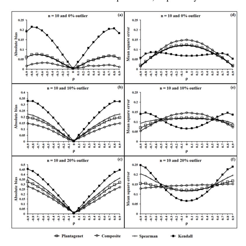
Figure 1 Estimates of absolute bias and mean square error of the four rank correlation coefficients for n = 10 and percentages of outliers in data y equal 0, 10 and 20.
The simulation results are shown in Figure 1 to Figure 4. Figures 1(a), 1(b) and 1(c) show that the ABSs of the proposed estimator, \(r_C\), had the smallest value both in the case of non-outliers and outliers in the data for a sample size of 10 and all levels of \(\rho\). In addition, the \(r_C\) tended to have the smallest MSE when ρ < -0.5 or ρ > 0.5 for a sample size of 10 and all percentages of outliers in the data, which are shown in Figures 1(d), 1(e) and 1(f). In the case of ρ is between -0.5 and 0.5 for a sample size of 10 and all percentages of outliers in the data, the MSEs of rK were lower than those of rC. However, the ABSs of rK had the largest value in this situation. In the case of non-outliers in the data and sample sizes of 30 and 50, the ABSs of rC, which are shown in Figures 2(a) and 3(a), seemed to have the smallest values. Moreover, the MSEs of rC, which are shown in Figures 2(d) and 3(d), were not greater than 0.05 in these situations. In the case of outliers in the data and sample sizes of 30, 50 and 100, the ABSs of rC and rPG, which are shown in Figures 2(b), 2(c), 3(b), 3(c), 4(b) and 4(c), seemed to be no different and had the smallest value for all levels of ρ.
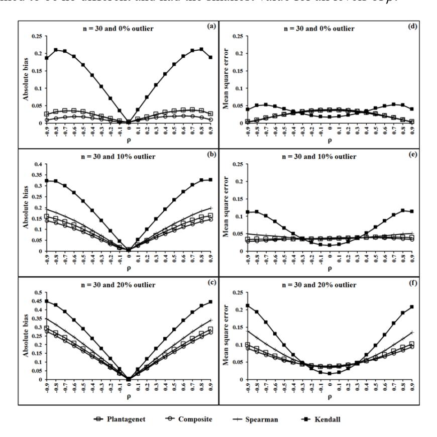
Figure 2 Estimate of absolute biase and mean square error of the four rank correlation coefficients for n = 30 and percentages of outliers in data y equal 0, 10 and 20.
For sample sizes of 30 and 50, the MSEs of the proposed estimator, rC, which are shown in Figures 2(d), 2(e), 2(f), 3(d), 3(e) and 3(f), tended to have the smallest values for almost all levels of , whatever the percentage of outliers in the data. For a sample size of 100 and non-outliers in the data, the ABSs of rC, rPG and rS, which are shown in Figure 4(a), seemed to have the smallest value for all levels of ρ. In addition, the MSEs of these three estimators, which are shown in Figure 4(d), were not greater than 0.05 and tended to have the smallest values in this situation.
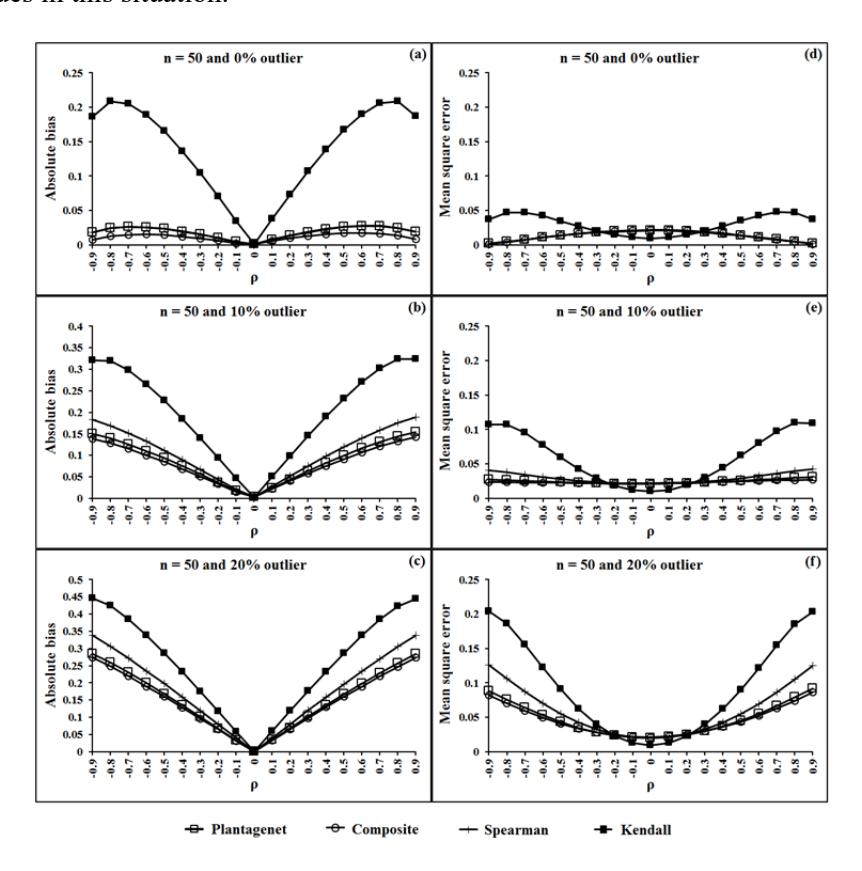
Figure 3 Estimate of absolute biase and mean square error of the four rank correlation coefficients for n = 50 and percentages of outliers in data y equal 0, 10 and 20.
When the data were contaminated with outliers and sample size of 100, which are shown in Figures 4(e) and 4(f), the MSEs of rC and rPG tended to have the smallest value for all level of ρ. In addition, Figures 1(a) to 4(a) show that the ABSs of almost all methods, except the Kendall' tau method, tended to decrease when the sample size increased and there were non-outliers in the data, but the MSEs of all methods, which are shown in Figures 1(d) to 4(d), tended to decrease.
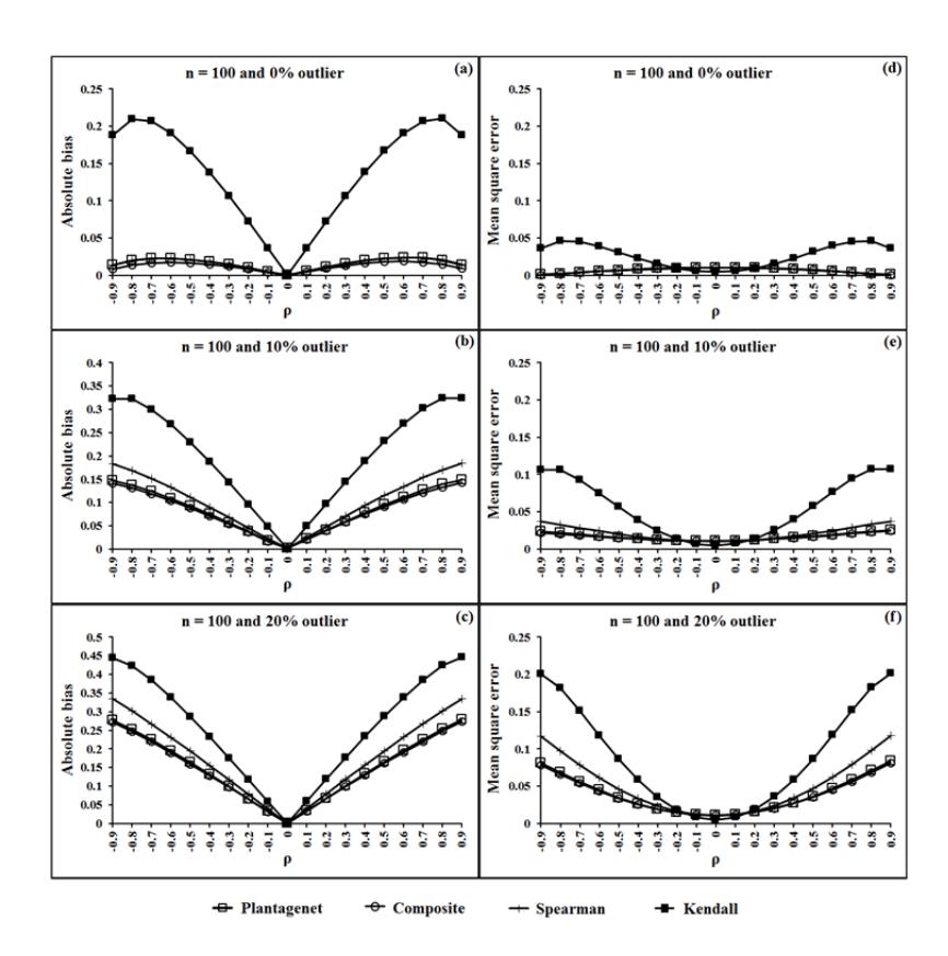
Figure 4 Estimate of absolute biase and mean square error of the four rank correlation coefficients for n = 100 and percentages of outliers in data y equal 0, 10 and 20.
In the case of outliers in the data, there were no effects of sample size with the ABSs of rC and rK, except for Plantagenet's and Spearman's rho correlation coefficients, where their ABSs tended to decrease when the sample size increased. Moreover, Figure 4 shows that the composite and Plantagenet's correlation coefficients seemed to have the same levels of ABS and MSE for a large sample size of 100, whatever the level of ρ and the percentage of outliers in the data, but the composite correlation coefficient was better than Plantagenet's correlation coefficient in terms of the ABSs, which are shown in Figures 1(a), 1(b) and 1(c) for a small sample size of 10, whatever the level of ρ and the percentage of outliers in the data. Moreover, Kendall's tau correlation coefficient seemed to have a large ABS in all situations studied. Additionally, the MSEs of all methods tended to decrease when the sample size increased with all percentages of outliers in the data. All methods seemed to have large ABS and MSE values when the percentage of outliers in the data increased for all sample sizes.
4 Discussion
The simulation results show that Spearman's rho and Kendall's tau correlation coefficients are not robust estimators when the percentage of outliers in the data increases, as mentioned by Abdullah [5]. Moreover, Kendall's tau correlation coefficient is heavily biased for most values of ρ, as mentioned in the studies of Evandt, et al. [12]. In this study, we found that Plantagenet's correlation coefficient is not sensitive to outliers, as studied by Maturi and Elsayigh [2].
5 Conclusion
The proposed estimator (a composite correlation coefficient) was derived based on a combination of Blest's and the adapted Blest's correlation coefficients with equal weighting between them. Furthermore, the jackknife procedure was applied for bias reduction when the data were contaminated with outliers. A simulation study was conducted to compare the efficiencies of the proposed estimator with three estimators. The good estimators that have small ABS and MSE values in each situation are shown in Table 1.
Table 1 Robust rank correlation coefficients for the bivariate normal distribution to resist outliers in the data for each situation.
| Sample Size (n) | Percentages of Outliers | ||
|---|---|---|---|
| 0 | 10 | 20 | |
| 10 | Composite | Composite | Composite |
| 30 | Composite | Composite | Composite |
| Plangenet | Plangenet | ||
| 50 | Composite | Composite | Composite |
| Plangenet | Plangenet | ||
| 100 | Composite | Composite | Composite |
| Plangenet | Plangenet | Plangenet | |
| Spearman | |||
Note: Composite = rC is robust estimator for all levels of ρ, Plantagenet = rPG is robust estimator for all levels of ρ, Spearman = rS is robust estimator for all levels of ρ.
The composite correlation coefficient seems to be the most robust estimator for all sample sizes and all levels of ρ, whatever the percentage of outliers in the data. This estimator can be calculated without difficultly by computer programming (see Appendix). In the case of outliers in the data, Plantagenet's correlation coefficient seems to be the most robust estimator for a large sample size (n = 30,50 and 100) and all levels of ρ. In the case of non-outliers in the data, the proposed composite correlation coefficient seems to perform well for all levels of the sample size and ρ.
Acknowledgements
This research was financially supported by the Kasetsart University Research and Development Institute (KURDI). The author would like to thank the head of the Department of Statistics, Faculty of Science, Kasetsart University for supplying the facilities necessary for the research.