
1 Introduction
The dynamics of equatorial Kelvin waves in the Indian Ocean have long been a subject of keen interest because of their critical role in thermocline adjustment [1]. Both observational and numerical studies have demonstrated that these nondispersive waves transmit signals rapidly across the ocean basin, affecting the sea level and sea surface temperature (SST) near the eastern boundary [2,3]. Recent observational and numerical studies [4,5] have shown that the wave activity shows strong intraseasonal variations and is driven primarily by intraseasonal winds over the central and eastern equatorial Indian Ocean.
Recently, it has been shown that the variability of the intraseasonal winds over the equatorial Indian Ocean is modulated by the Indian Ocean Dipole (IOD) on interannual timescales [6,7]. This suggests the existence of interesting scale-interactions among shorter- and longer-period phenomena in the tropical Indian Ocean. During the IOD event, the westerly zonal winds are anomalously weakened or even reversed in direction [8]. This leads to absence of eastward equatorial oceanic jets in the Indian Ocean and contributes to lowering (shoaling) the sea level (thermocline) in the eastern Indian Ocean and rising (deepening) the sea level (thermocline) in the western Indian Ocean [9,10]. This east-west zonal tilt of the thermocline along the equator may have an influence on the characteristics of the Kelvin waves [11,12].
Sometimes intraseasonal variability may upset IOD evolution, which was the central focus of the predictability study reported in [13]. However, in the present study the focus is on determining to what extent the spatio-temporal variations in the background stratification during an IOD event influence the characteristics of intraseasonal Kelvin waves. In particular, we discuss two typical IOD events: the pure IOD in 1994 and the IOD co-occurring with El Niño in 1997/98.
2 Methods and Ocean Model
2.1 Methods
We start from the linear shallow-water equations [14], written as
\[u_{t} - fv + \frac{1}{\rho_{o}} p_{x} = \frac{1}{\rho_{o}} X_{z}\] (1)
\[v_t + fu + \frac{1}{\rho_o} p_y = \frac{1}{\rho_o} Y_z \tag{2}\]
\[p_z = -\rho g \tag{3}\]
\[u_x + v_y + w_z = 0 (4)\]
\[\rho_t + w \rho_z = 0 \tag{5}\] where suffixes t, x, y and z indicate the partial derivative with respect to these variables. (X, Y) indicates the external forces such as wind stress and (u, v, w) are the zonal, meridional and vertical velocity, respectively. The parameters p, f and g indicate the pressure, the Coriolis parameter and the acceleration due to gravity, respectively. The parameter \(\rho_o\) is the reference density. The equation of motion is then simplified to its vertical mode, in which the structure function \(\psi_n(z)\) is determined by
\[\left(\frac{\psi_{nz}}{N^2}\right)_z + \frac{1}{c_n^2}\psi_n = 0 \tag{6}\] with boundary conditions \(\left(\frac{\psi_{nz}}{N^2}\right)_z + \frac{\psi_n}{g} = 0\) at z = 0 and \(\psi_{nz} = 0\) at z = -D
(bottom depth) and normalized so that \(\psi_n(0) = 1\), where \(N = \sqrt{-g \frac{\overline{\rho_z}}{\rho_o}}\) is the
Brunt-Väisälä frequency and \(c_n\) is the eigenvalue (the phase speed of the nth mode).
The horizontal velocity and the pressure can be expanded as
\[q = \sum_{n=0}^{\infty} q_n(x, y, t) \psi_n(z)\] (7)
where q denotes u, v or p. Similarly, the vertical velocity is expanded as
\[w_z = \sum_{n=0}^{\infty} w_n(x, y, t) \psi_n(z), \qquad (8)\] and the external forcing can also be expanded as
\[\frac{1}{\rho_o}(X,Y) = \sum_{n=0}^{\infty} \left(X_n(x,y,t), Y_n(x,y,t)\right) \psi_n(z). \tag{9}\]
By substituting Eq. (7)-(9) into Eq. (1)-(5), we find equations for each vertical mode
\[u_{nt} - fv_n + p_{nx} = X_n (10)\]
\[v_{nt} + fu_n + p_{nv} = Y_n \tag{11}\]
\[\frac{1}{c_n^2} p_{nt} + u_{nx} + v_{ny} = 0, (12)\] where \((X_n, Y_n)\) are given by
\[(X_n, Y_n) \int_{-D}^{0} \psi_n^2 dz = \int_{-D}^{0} \frac{1}{\rho_o} (X_z, Y_z) \psi_n dz.\] (13)
Assuming that (X, Y) decreases linearly from its surface value \((\tau^x, \tau^y)\) to zero at the mixed layer depth \(H_{mix}\), such that
\[(X_z, Y_z) = \begin{cases} \frac{(\tau^x, \tau^y)}{H_{mix}} & -H_{mix} < z < 0\\ 0 & z < H_{mix} \end{cases}\](14)
Note that the mixed layer depth \((H_{mix})\) is estimated as a depth at which the density is 0.2 kg m<sup>-3</sup> larger than the surface density [15]. The Eq. (13) is, then, simplified to
\[(X_n, Y_n) = \frac{B_n(\tau^x, \tau^y)}{\rho_o},\tag{15}\] where \(B_n\) is called as the equivalent forcing depth, which indicates how well the corresponding mode is coupled to the wind forcing. It is explicitly written as
\[B_n = \frac{\int\limits_{-H_{mix}}^{0} \psi_n(z)dz}{H_{mix} \int\limits_{-D}^{0} \psi_n^2(z)dz}.\] (16)
2.2 Description and Validation of Ocean Model
We have used outputs from a high-resolution OGCM developed for the Earth Simulator (OFES) [16]. The model, covering the region between 75°S to 75°N with a horizontal resolution of 1/10°, is based on the Modular Ocean Model (MOM3) code. There are 54 levels in the vertical, 17 of which are in the upper 150 m. Vertical mixing is based on the K profile parameterization (KPP) boundary layer mixing scheme, while horizontal mixing uses a bi-harmonic smoother. The surface salinity field is restored to climatological monthly mean values of WOA98 with a timescale of 6 days. Also, surface heat and fresh water flux are specified using bulk formula with an atmospheric data set obtained from the monthly mean climatology of NCEP/NCAR reanalysis data [17]. The model is integrated for 54 years, from January 1950 to December 2003, using the daily mean NCEP/NCAR reanalysis data.
Figure 1 compares model and observational results for the intraseasonal (20-100-day) subsurface zonal current at 0°N, 90°E for the period of January 2001 to December 2003. It can be seen that the model reproduces the observed features very well. At all levels the correlation coefficients are larger than 0.5 (significant at a 95% confidence level).
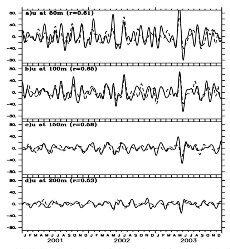
Figure 1 (a) 20-100-day band-passed time series of the observed (solid) and model (dashed) zonal currents (cm/s) in the eastern equatorial Indian Ocean (0°N, 90°E) during January 2001 – December 2003 at 50-m depth. (b)-(d) Same as (a) except for currents at 100-m, 150-m and 200-m depth, respectively.
However, the model generally underestimates the strong eastward currents associated with the spring Yoshida-Wyrtki jet. Nevertheless, a good level of agreement between the simulated and observed surface and subsurface oceanic variabilities suggests that model is sufficiently accurate to capture the interannual modulation of the intraseasonal oceanic variations associated with IOD events. Results from the last 14 years of the simulation (1990-2003) were used in the following analysis.
3 Results
3.1 Spectral Characteristics
Variance spectra of observed SSH from TOPEX/Poseidon, model SSH and depth of 20 °C isotherm (D20), and observed zonal wind stress along the equator in the Indian Ocean are displayed in Figure 2.
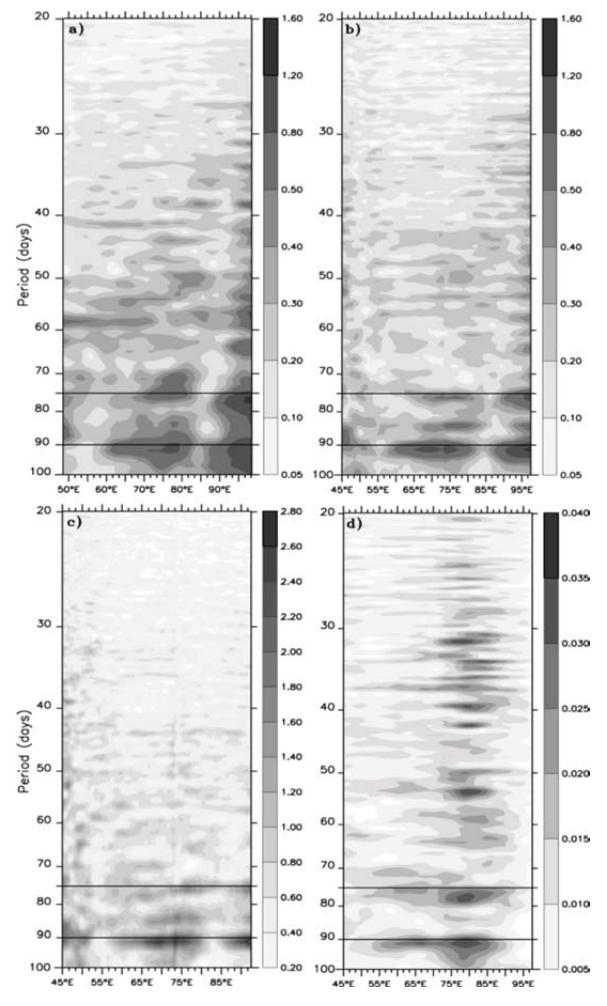
Figure 2 Variance-preserving spectra of (a) observed sea surface height from TOPEX/Poseidon (cm²), (b) model sea level (cm²), (c) model depth of 20 °C isotherm (m²) and (d) observed zonal wind stress (dyn² cm²) along the equatorial Indian Ocean (averaged over 1°S-1°N). The spectra were calculated based on a 10-year record (1993-2002) from TOPEX/Poseidon and a 14-year period (1990-2003) for other fields.
Although the intraseasonal variations in both observed and modeled SSH appear as a relatively energetic band with periods from 40 to 100 days, maximum energy is confined around the periods of 75 and 90 days (Figures 2(a-b)). These peaks are also evident in the spectra of D20 and well distinguished from intraseasonal variations at higher frequencies (Figure 2(c)). We note that the energy in the 75- and 90-day bands are more prominent in the central and eastern Indian Ocean for both SSH and D20.
Corresponding spectral peaks are also prominent in the observed zonal wind stress (Figure 2(d)), suggesting influence of wind forcing on the equatorial waves. Several studies have also pointed out the importance of wind forcing in generating oceanic variations within the intraseasonal timescale [3-5]. Given that the intraseasonal variations with the periods of 75 and 90 days are a prominent feature of intraseasonal variability of all fields (Figures 2(a-d)), our analysis in the rest of the paper will focus on those frequency bands.
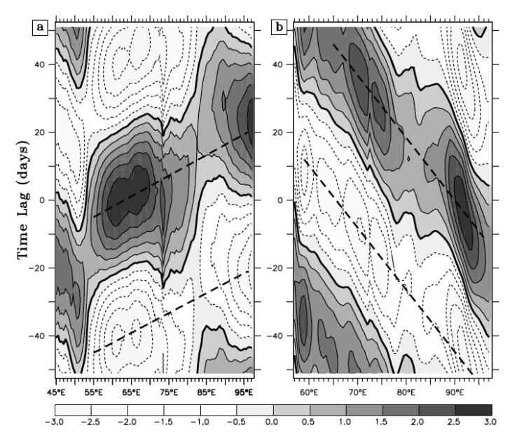
Figure 3 Composite of 70-100 day filtered D20 (a) along the equator, and (b) along 5ºS. The dashed lines estimate trajectories of the propagating signals.
In order to evaluate the dynamics of 75-95-day variations, we calculated a composite average of band-pass filtered D20. A band-pass filter with cut-off periods of 70-100 days was applied to the simulated D20 field. We began our calculation by developing indices for the signals both along the equator (hereafter Kelvin wave index) and along 5S (hereafter Rossby wave index). The Kelvin wave index is defined as band-pass filtered D20 maxima at 65°E, while the Rossby wave index is denoted as band-pass filtered D20 maxima at 92°E. Then, the dates of every positive maxima of both Kelvin and Rossby wave indices were identified, which resulted in 57 and 59 events, respectively (significant at 95% confidence limit). Finally, the band-pass filtered D20 values were averaged over those dates and a range of time lags. The results gave values of 2.15 m s-1 and 0.69 m s-1 for the eastward- and westward-propagating signals, as shown in Figures 3(a) and 3(b) respectively.
The former was compared with theoretical phase speeds derived from the model density profile and the mean density profile of the monthly gridded ARGO floats data (Table 1) [18]. Since the estimated phase speeds from the composite analysis fall between the theoretical values of the first and the second baroclinic mode, this may indicate that both modes are present in the 75-95-day oceanic variations in the equatorial Indian Ocean.
Table 1 Phase Speed (m s-1) based on Mean Model Density Profiles 1990- 2003.
| No | 50°E | 60°E | 70°E | 80°E | 90°E |
|---|---|---|---|---|---|
| 1 | 2.51 (2.71) | 2.52 (2.74) | 2.52 (2.70) | 2.54 (2.80) | 2.56 (2.86) |
| 2 | 1.60 (1.63) | 1.62 (1.66) | 1.63 (1.67) | 1.68 (1.76) | 1.71 (1.80) |
| 3 | 0.88 (0.98) | 0.88 (0.99) | 0.88 (0.99) | 0.89 (1.01) | 0.88 (1.02) |
| 4 | 0.60 (0.72) | 0.62 (0.74) | 0.63 (0.74) | 0.63 (0.74) | 0.65 (0.74) |
| 5 | 0.52 (0.58) | 0.54 (0.59) | 0.55 (0.58) | 0.55 (0.59) | 0.56 (0.60) |
Note: Values in brackets were obtained from the mean density fields of gridded ARGO data.
3.2 Interannual Modulation of Baroclinic Modes
To examine the interannual modulation of the intraseasonal Kelvin waves, the band-passed filtered simulated D20 was evaluated. First, the phase speed of the intraseasonal Kelvin waves for three different periods was calculated: January 1999 – December 2000, September 1997 – March 1998, and July – December 1994. Each period represents normal conditions, the IOD co-occurring with El Niño, and the pure IOD conditions, respectively.
Table 2 Phase Speed (m s-1) of Kelvin and Rossby Waves during IOD Conditions.
| Period | Kelvin waves | Rossby waves |
|---|---|---|
| a. October 1997 – April 1998 | ||
| October – November 1997 | 2.38 | 0.22 |
| November – December 1997 | 2.34 | 0.20 |
| December 1997 – January 1998 | 1.59 | 0.19 |
| February – March 1998 | 1.02 | 0.19 |
| March – April 1998 | 0.93 | 0.19 |
| b. July – December 1994 | ||
| July – August 1994 | 0.91 | 0.18 |
| September – October 1994 | 1.02 | 0.14 |
| October – November 1994 | 1.08 | 0.19 |
| November – December 1994 | 1.21 | 0.19 |
The phase speed for normal conditions without IOD event was obtained by calculating a composite averaged of band-pass filtered D20 over this period. The results suggest phase speeds of about 2.33 m s-1 and 0.7 m s-1 for Kelvin and Rossby waves, respectively. On the other hand, the phase speeds during IOD conditions were estimated using the slopes of the trajectory lines in the time-longitude diagrams of band-pass filtered D20 over the same periods (Figures 4 and 5); the results are listed in Table 2. It is apparent that the phase speeds of the intraseasonal Kelvin waves decreased during the IOD years compared to those during a normal year. During the IOD co-occurring with El Niño in 1997/98, the phase speed decelerated from 2.38 m s<sup>-1</sup> in October – November 1997 to 0.93 m s<sup>-1</sup> in March – April 1998 (Figure 4(a)).
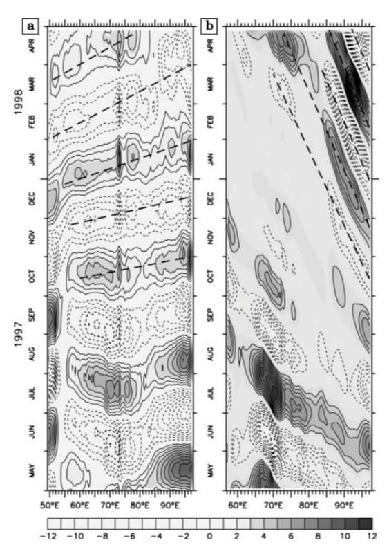
Figure 4 Time-longitude diagrams of 70-100-day filtered D20 (m) along the equator (a) and along 5°S (b) for the period of May 1997 – April 1998. The zero contour is omitted and the dashed lines represent trajectories of the propagating signals.
Meanwhile, during the pure IOD condition in 1994, the phase speed increased from 0.91 m s<sup>-1</sup> in July – August 1994 to 1.21 in November – December 1994 (Figure 5(a)). Since the phase speeds of the intraseasonal Kelvin waves during IOD conditions, both in 1997/98 and in 1994, do not correspond exactly to the theoretical values listed in Table 1, this suggests that the waves seem to involve several modes.
The phase speed of the Rossby waves also significantly decreased during the IOD conditions compared to those during normal conditions. The dashed lines in Figures 4(b) and 5(b) indicate westward propagation with phase speeds between 0.14 and 0.22 m s-1. Assuming that these westward-propagating signals were associated with the first meridional (ℓ = 1) Rossby waves, corresponding eastward propagation Kelvin wave speeds between 0.42 and 0.66 m s-1 were obtained. This range of phase speeds falls between the theoretical values of the fourth and the fifth baroclinic modes (see Table 1).
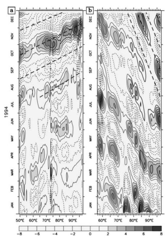
Figure 5 Same as Figure 4 except for the period of January – December 1994.
To further examine which baroclinic modes are involved in the intraseasonal Kelvin waves normal mode decomposition is useful. Using Eq. (7), the contribution of each baroclinic mode to the intraseasonal pressure along the equator can be calculated. Note that the decomposition of the normal mode is based on the mean stratification of the respective events. The calculation of the vertical mode for normal years is based on the mean stratification of January 1999 – December 2000, while that for the 1997/98 and 1994 IOD events was calculated based on the mean stratification of September 1997 – March 1998 and July – December 1994, respectively. Figure 6 compares the explained
variance of the first four baroclinic modes relative to the total intraseasonal pressure for three typical periods. The joint contribution of the first four modes as well as that of the first six modes is also presented.
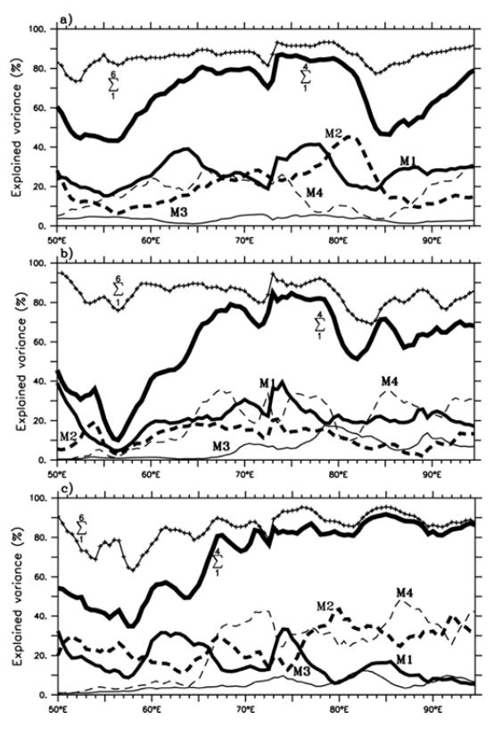
Figure 6 (a) Explained variance along the equator referenced to the 70-100-day band-passed pressure for mode 1 contribution (thick line), mode 2 (thick dashed line), mode 3 (thin line), mode 4 (thin dashed line), sum of the first four modes (extra thick line) and sum of the first six modes (crossed line). The vertical mode decomposition is based on the mean density profiles for January 1999 – December 2000. For (b) and (c) same as in (a) except for the mean density of September 1997 – March 1998 and July – December 1994, respectively.
During normal conditions, the intraseasonal variations along the equator mostly involve the first two baroclinic modes (Figure 6(a)), while the first mode explains a large variance at longitude of 60-65ºE, 75-80ºE and east of 85ºE (~30–40% of the total variance), the second mode has maximum variance around 82ºE (about 40% of the total variance). The fourth mode presents variance peaks in the central (65-75ºE) and eastern (east of 89ºE) basin, reaching ~20% of the total variance. The contribution of the first four modes to the total variance in the central basin from 60º to 83ºE is significantly high (> 60%), indicating only a small contribution from the higher modes.
The situation is different for the 1997/98 IOD event; the variance explained by the fourth mode significantly increases, reaching ~40% of the total variance in the central (65-80ºE) and eastern (east of 85ºE) basin (Figure 6(b)). The variance explained by the first mode reduces in the eastern and western basin, while in the central basin (around longitude of 75ºE) it still explains about 35% of the total variance. Moreover, the joint contributions of the first four modes around 57°E drops to ~20% of the total variance. This indicates that contributions from the higher modes are required to explain the total variance there. On the other hand, in the eastern basin between 80ºE and 90ºE, the joint contribution of the first four modes is higher compared to that during a normal year.
During the 1994 IOD event, the fourth mode explains up to 45% of the total variance in the eastern basin east of 85ºE. In the central basin, between 75ºE and 85ºE, the second mode explains about 40% of the total variance (Figure 4(c)). The variance explained by the first mode is weak in the eastern basin but increases up to ~30% around 75ºE and between 60ºE and 66ºE. The percentage of the variance explained by the sum of the first four modes east of 65ºE is high (~80%) but in the western basin west of 65ºE it is low.
3.3 Equivalent Forcing Depth
The differences in the baroclinic modal contributions of the intraseasonal pressure along the equator were further investigated by calculating the equivalent forcing depth for each baroclinic mode using Eq. (16). Similar to the calculation of pressure variation shown in Figure 6, the equivalent forcing depth is based on the mean stratification of the respective event (e.g. normal year and IOD year). The results illustrated in Figure 7 suggest that the equivalent forcing depth varies with the IOD conditions.
Under normal conditions, the wind forcing is mostly projected onto the two gravest modes, among which the second mode is more efficiently excited than the first mode (Figure 7(a)). However, the equivalent forcing depth of the first mode increases gradually toward the east, while that of the second mode decreases. The third mode remains weak across the basin, while the fourth mode shows zonal variations with maxima in the central basin between 60°E and 75°E, and near the eastern boundary.
Under IOD conditions in 1997/98 and 1994, the equivalent forcing depth of the fourth baroclinic mode significantly increases, particularly near the eastern
boundary (Figures 7(b-c)). This means that the fourth mode is strongly excited near the eastern boundary by winds under IOD conditions. The equivalent forcing depth of the first mode decreases slightly toward the east, while that of the second mode increases. These characteristics of the first two modes during IOD conditions are in contrast with those during normal conditions.
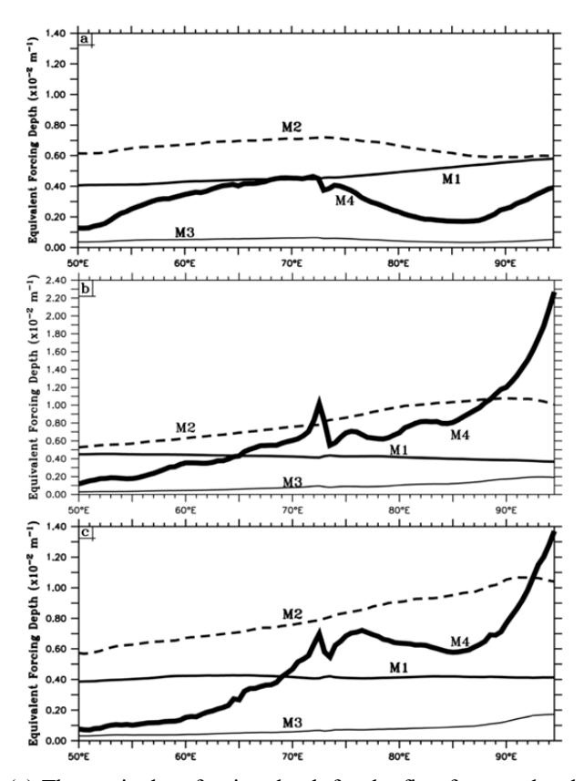
Figure 7 (a) The equivalent forcing depth for the first four modes derived from the vertical mode decomposition over the period of January 1999 – December 2000. (b)-(c) Same as in (a) except calculated over the period of September 1997 – March 1998, and July – December 1994, respectively. Note the scale change for the 1997/98 IOD event.
The spatial variation of the equivalent forcing depth does not correspond exactly with the spatial variation of the baroclinic modal contributions (see Figure 6). Note that the calculation of the equivalent forcing depth requires temporal vertical mode and mixed layer depth, which were not adopted in this study. In addition, it is known that the equivalent forcing depth solely depends on local forcing, while pressure variation can be excited by many factors, such as wave-current interactions, wave propagation and reflection, and damping.
On the other hand, the temporal variation of the equivalent forcing depth is consistent with variations of the baroclinic modal contributions. One possible explanation for these variations lies in the temporal variations in the background stratification. A previous study [11] pointed out that the wind generates efficiently higher baroclinic modes in regions where the pycnocline is sharp as well as shallow.
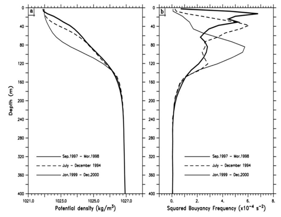
Figure 8 (a) Vertical profiles of the potential density averaged over the region of (80-90°E, 1°S-1°N) and computed over the period of January 1999 – December 2000 (thin solid line), September 1997 – March 1998 (thick solid line), and July – December 1994 (dashed line), (b) The corresponding vertical profiles of the Brunt-Väisälä frequency.
To clarify, both the vertical structure of the potential density and the Brunt-Väisälä frequency averaged over the eastern equatorial Indian Ocean (80-90°E, 1°S-1°N) are shown in Figure 8. We find a significant difference in the vertical profile of the pycnocline between normal and IOD conditions (Figure 8(a)). During IOD events, the pycnocline is shallowed by about 50 m. Consequently, the vertical stratification in the surface layer (~20 m during 1997/98 and ~40 m during 1994) is significantly intensified, while at a lower level (~100 m) it is conversely weakened (Figure 8(b)). In the western basin, however, the vertical structure of the potential density and that of the Brunt-Väisälä frequency experience only small change (not shown).
4 Conclusion
In this study, a high-resolution OGCM was used to examine the impact of IOD events on the characteristics of intraseasonal Kelvin waves along the equatorial Indian Ocean. The analysis was focused on the variability of the vertical structure of intraseasonal Kelvin waves.
During normal conditions, the vertical modal decomposition suggests that the first two modes dominate the variation. The contribution from the first mode was high (~35-40%) at longitudes of 60-65ºE and 75-80ºE, while the second mode was more dominant in the central basin around a longitude of 82ºE contributing about 40% to the total variance.
During IOD events, the pycnocline in the eastern basin was raised by about 50 m and the stratification at the upper level was strengthened, while that at the lower level was weakened. All these changes have an impact on the dominant modes composing the intraseasonal Kelvin waves. We found that during the 1997/98 IOD event, the contribution from the fourth baroclinic mode significantly increased in the central (65-80ºE) and eastern (east of 85ºE) equatorial Indian Ocean, explaining ~40% of the total variance. During the 1994 IOD event, the fourth baroclinic mode, explaining ~45% of the total variance, was still the leading mode in the eastern basin. However, in the central basin between 75ºE and 85ºE, the second mode contributes almost the same variance (~40%) as the fourth mode.
The above finding demonstrates the dependence of the higher order mode's contribution to temporal as well as spatial variations of density structures. We note that the contribution significantly varies in the eastern equatorial Indian Ocean off Sumatra. In addition to the change of the vertical stratification, change in the mean current may also influence the characteristics of intraseasonal Kelvin waves. During IOD events, the surface current in the upper 50 m is anomalously westward. A previous study [19], using a numerical model, found that the presence of the mean current does modify the characteristics of the Kelvin waves. The effect depends on the speed and vertical and meridional structures of the mean current. In contrast to the first baroclinic mode that experiences only a weak Doppler shift because its structure is similar to the mean current, higher baroclinic modes are more clearly influenced by the Doppler effect. However, how the change of the mean current associated with an IOD event influences the characteristics of the intraseasonal Kelvin waves awaits further analysis.
Acknowledgements
The authors benefited from discussions with Prof. T. Yamagata, Prof. Y. Masumoto, Drs. T. Tozuka, S.K. Behera, and S.A. Rao. The OFES simulation was conducted using the Earth Simulator by Dr. H. Sasaki. The NOAA/PMEL Ferret program was used to generate the figures. The wavelet software was provided by Drs. C. Torrence and G. Compo. This research was financially supported by a Grant for Scientific Research from the University of Sriwijaya (Hibah Kolaborasi Internasional) and from the Ministry of Research, Technology and Higher Education, Republic of Indonesia (Hibah Kompetensi, No: 023/SP2H/LT/DPRM/II/2016).