
1 Introduction
The Generalized Space Time Autoregressive (GSTAR) model can be used to forecast several locations simultaneously with a sequence of observations based on time. For example, the exchange rate of the dollar against a number of currencies in a region. The research development of this model is attractive, either for mathematical modeling or for applications. In GSTAR modeling, the error assumption must be considered, since it can influence the estimation of the model parameters. It is common to assume that the errors are independent with identically normal distribution, as is often the case in time-series modeling. More challenging in modeling space-time observations is forecasting future values in unobserved locations. This can be done by combining GSTAR and kriging modeling, which gives better results than combining time-series and kriging modeling [1].
If spatial dependence among locations exists, then involving this dependence as early as possible is better. Furthermore, there is a chance that dependence not only exists between observations temporally or spatially but also between errors. Because of this, the independent error assumption is not always satisfactory for data that have a dependency in errors in time and/or space.
Several researchers have done work in the field of error assumption. Nurhayati [2] has developed a spatially correlated error assumption for the GSTAR(1;1) model, while Fadlilah, et al. [3] defined the martingale difference process as a cross product of two consecutive errors. Both assumptions maintain the linear model form of the GSTAR(1;1) process, so that the 'family' of least squares estimation can still be applied. GSTAR models have been widely applied in various fields. Nurhayati, et al. [4] applied GSTAR(1;1) to GDP data of European countries. Mukhaiyar and Pasaribu [5] identified the GSTAR(2;3,0) model for the monthly tea production of a number of plantations in West Java through the new Inverse of Autocovariance Matrix (IAcM) approach. Fadlilah, et al. [3] applied GSTAR(1;1) to weekly red-chili prices in traditional markets in Bandung. The first two applications considered an independent and normal distribution of errors, while the last one considered temporally correlated errors.
This paper is divided into six sections. Section 2 briefly explains GSTAR as well as the different ways of selecting spatial weights. Section 3 examines GSTAR with various errors assumptions, from an independent (uncorrelated) identical normal distribution of errors to dependence of errors, both temporally and spatially correlated. Our simulation study is discussed in Section 4. Application of this model with each of the assumptions is discussed in Section 5. Conclusions and remarks are put forward in Section 6.
2 GSTAR
GSTAR is a special form of the vector autoregressive (VAR) model. A process vector at time t, \(\mathbf{Y}(t) = (Y_1(t), Y_2(t), ..., Y_N(t))'\), which involves N spatial locations, follows the GSTAR process p-time order and spatial order \(\lambda_1, \lambda_2, ..., \lambda_p\)
, written as GSTAR ( \(p; \lambda_{ _{1}}, \lambda_{ _{2}}, ..., \lambda_{ _{p}} )\) [6] if
\[Y_{i}(t) = \sum_{k=1}^{p} \left( \phi_{k0}^{(i)} Y_{i}(t-k) + \sum_{\ell=0}^{\lambda_{k}} \phi_{k\ell}^{(i)} \sum_{j=1}^{N} w_{ij}^{(\ell)} Y_{j}(t-k) \right) + \varepsilon_{i}(t)\] for \(i = 1, 2, ..., N; t = 1, 2, ..., T\) (1)
with k: autoregressive time order k = 1, 2, ..., p
\(\ell\): spatial autoregressive/location order \(\ell = 0, 1, 2, ..., \lambda_k\)
\(\varepsilon_i(t)\) : errors at time t on location i
\(w_{ij}^{(\ell)}\): spatial weight location j related to location i in the \(\ell\)-th spatial order \(\emptyset_{k\ell}^{(i)}\): autoregressive parameters for k-time order and the \(\ell\)-th spatial order
The GSTAR modeling follows Box-Jenkins' three stages of time-series analysis. These are: model identification, parameter estimation and diagnostic checking. Identifying the space-time model is carried out with the STARMA model by Pfeifer and Deutsch [7], which uses the space-time autocorrelation function (STACF) and the space-time partial autocorrelation function (STPACF). In time-series analysis both of these functions are similar to the autocorrelation function (ACF) and the partial autocorrelation function (PACF).
In space-time analysis, the spatial weights of the model greatly affect the parameter estimation, which distinguishes it from time-series analysis. Until now, the selection of spatial weights is subjective, depending on the researcher. There are several ways of selecting the weights to be used: with uniform, binary and non-uniform weight [5], based on the distance matrix and the inference of cross correlation [8], where weighting of locations can be done by normalization of the cross correlation magnitudes between locations during the corresponding process. In addition, by defining the spatial weights, the level of geographical adjacency between two locations is quantified, which is a major feature of the space-time model. This spatial weighting then establishes a well-defined weight matrix for each observed spatial lag. The spatial weight value starts from zero and goes to one. Zero indicates the loosest relationship between two observed locations, while one indicates the closest relationship.
For simplicity, a uniform weight was chosen for the GSTAR modeling in this study. Location grouping at uniform weight was carried out by order of the distance between two locations. The weight was determined based on the numbers of neighbor locations within a certain spatial lag for a certain location.
This is expressed as \(w_{ij}^{(\ell)} = \frac{1}{n_i^{(\ell)}}\), where i is a neighbor of j and zero in all other
cases, where \(n_i^{(\ell)}\) is the number of the nearest neighbors of location i in the same spatial lag \(\ell\).
3 Estimation of GSTAR Model Parameters
One of the most important stages in modeling is the parameter estimation. The general procedure of space-time modeling is shown in Figure 1. This procedure was taken from Mukhaiyar and Pasaribu [5] and slightly modified regarding parameter estimation. The least squares method is commonly used in the estimation stage but it is only effective for GSTAR with independent error assumption. Correlated error assumption, both temporal and spatial, requires another method, such as the generalized least squares (GLS) method.
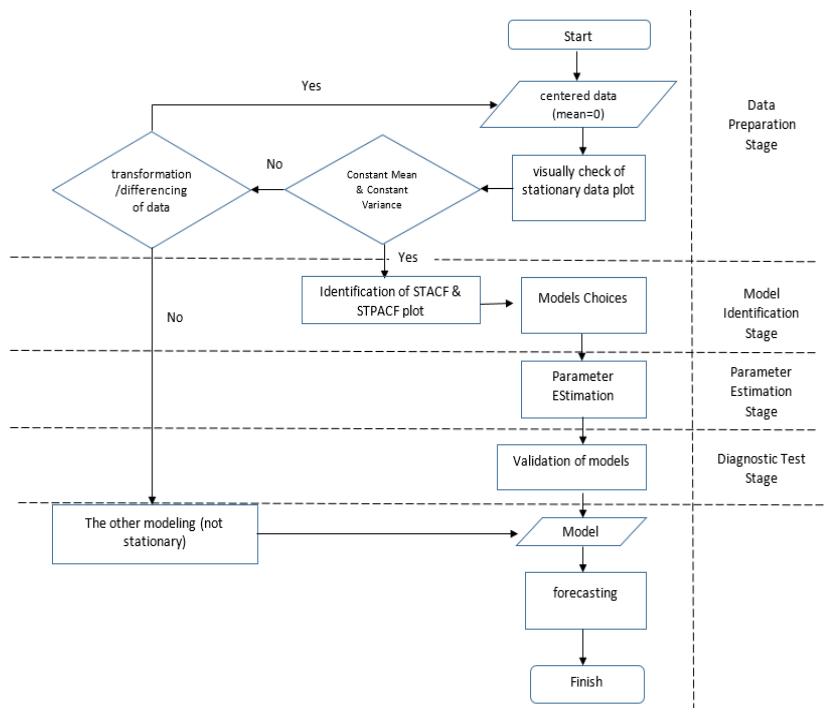
Figure 1 Procedure of space-time modeling. This procedure adopts Box-Jenkins' three iterative stages of time-series analysis.
3.1 Uncorrelated Errors (Independent Errors)
GSTAR parameter estimation with error independence assumption can be conducted using the least squares (LS) method. This method is widely used for linear models. LS estimators obtained by minimizing the sum of squares of errors are commonly used in regression models and have been proven in the GSTAR(1;1) model [2].
There are several assumptions regarding errors that need to be considered when using LS. Independent errors with zero mean and constant variance are the main assumptions used, beside normal distribution. From Eq. (1), where \(p=1,\ \lambda_1=1\), the GSTAR(1;1) model can be derived as:
\[Y_{i}(t) = \phi_{0i}Y_{i}(t-1) + \phi_{1i}\left(\sum_{j=1}^{N} w_{ij}Y_{j}(t-1)\right) + \varepsilon_{i}(t), \ i = 1, 2, ..., N; \ t = 1, ..., T\] (2)
where \(\phi_{0i}\) and \(\phi_{1i}\) are autoregressive parameters of zero and first spatial lag, respectively, for the first time lag in location i. Furthermore, \(w_{ij}\) implies the influence of location j on location i at the first spatial lag. The model expressed in Eq. (2) can be seen as a multiple linear regression model with random covariates
\[\mathbf{Y} = \mathbf{X}\boldsymbol{\Phi} + \boldsymbol{\varepsilon} \tag{3}\] with
\[\mathbf{Y} = \begin{pmatrix} Y_i(1) \\ Y_i(2) \\ \vdots \\ Y_i(T) \end{pmatrix}, \mathbf{X} = \begin{pmatrix} Y_i(0) & V_i(0) \\ Y_i(1) & V_i(1) \\ \vdots & \vdots \\ Y_i(T-1) & V_i(T-1) \end{pmatrix}, \boldsymbol{\varPhi} = \begin{pmatrix} \phi_{0i} \\ \phi_{1i} \end{pmatrix}, \boldsymbol{\varepsilon} = \begin{pmatrix} \varepsilon_i(1) \\ \varepsilon_i(2) \\ \vdots \\ \varepsilon_i(T) \end{pmatrix},\] and \[V_i(t) = \sum_{j=1}^{N} w_{ij} Y_i(t)\] \(t = 1, 2, ..., T; i = 1, 2, ..., N\).
Since \(\mathcal{E}_i(t)\), the model is assumed to be identical, independent and normally distributed with zero mean and constant variance \(\sigma^2\), such that the vector of errors is \(\varepsilon \sim N(0, \sigma_\varepsilon^2 \mathbf{I}_{NT})\). The LS estimator for vector \(\phi\) is
\[\hat{\boldsymbol{\phi}} = (\mathbf{X}'\mathbf{X})^{-1}\mathbf{X}'\mathbf{Y} \tag{4}\]
This estimator is unbiased and has the smallest variance among the other unbiased linear estimators.
Theorem 1. [6] Estimation vector LS \(\hat{\phi}\) as defined in Eq. (4) is an unbiased estimator and has the smallest variance in the set of unbiased linear estimators.
Proof. Let \(\hat{\phi} = (\mathbf{X}'\mathbf{X})^{-1}\mathbf{X}'\mathbf{Y}\) be an LS estimator. Since \(\mathbf{\varepsilon} \sim \mathrm{N}(\mathbf{0}, \sigma_{\varepsilon}^2\mathbf{I}_{NT})\), we can write \(E[\varepsilon] = 0\). Given that the error vector \(\mathbf{\varepsilon}(t)\) does not correlate with the observation vectors in the past, as gathered in the explanatory matrix \(\mathbf{X}\), the conditional expectation error vector \(E[\mathbf{\varepsilon} \mid \mathbf{X}] = \mathbf{0}\). We can write
\[E \left[ \hat{\Phi} - \Phi \mid \mathbf{X} \right] = (\mathbf{X}'\mathbf{X})^{-1}\mathbf{X}'E \left[ \mathbf{\epsilon} \mid \mathbf{X} \right] = \mathbf{0}.\]
In other words, this shows that \(\widehat{\Phi}\) is an unbiased estimator for \(\Phi\). Furthermore, we may obtain that \(\widehat{\Phi}\) has the smallest variance in the set of unbiased linear
estimators. Suppose that \(\widehat{\Phi}^*\) is an unbiased estimated estimator for \(\Phi\) then \(E\left[\widehat{\phi^*} - \phi \mid \mathbf{X}\right] = \mathbf{0}\). We take
\[\widehat{\Phi^*} = (\mathbf{X}'\mathbf{X})^{-1}\mathbf{X}'\mathbf{Y} + \mathbf{U}\mathbf{Y}\]\[= ((\mathbf{X}'\mathbf{X})^{-1}\mathbf{X}' + \mathbf{U})\mathbf{Y}\]\[= \mathbf{H}\mathbf{Y}\] for the U function matrix of X, so we have
\[cov(\widehat{\phi}^* \mid \mathbf{X}) = E[(\mathbf{HY} - E[\mathbf{HY}])(\mathbf{HY} - E[\mathbf{HY}])' \mid \mathbf{X}]\] \[= E[\mathbf{H}(\mathbf{Y} - E[\mathbf{Y}])(\mathbf{Y} - E[\mathbf{Y}])' \mathbf{H}' \mid \mathbf{X}]\] \[= \mathbf{H}cov(\mathbf{Y}|\mathbf{X})\mathbf{H}'\] \[= \sigma_{\varepsilon}^{2}((\mathbf{X}'\mathbf{X})^{-1}\mathbf{X}' + \mathbf{U})(\mathbf{X}'\mathbf{X})^{-1}\mathbf{X}' + \mathbf{U})')\] \[= \sigma_{\varepsilon}^{2}((\mathbf{X}'\mathbf{X})^{-1}\mathbf{X}'\mathbf{X}(\mathbf{X}'\mathbf{X})^{-1} + \mathbf{U}'\mathbf{X}(\mathbf{X}'\mathbf{X})^{-1} + (\mathbf{X}'\mathbf{X})^{-1}\mathbf{X}'\mathbf{U}' + \mathbf{U}\mathbf{U}')\] \[= \sigma_{\varepsilon}^{2}((\mathbf{X}'\mathbf{X})^{-1} + \mathbf{U}\mathbf{U}').\]
Since each of the diagonal entries of UU' have a quadratic form, it is a positive semi-definite matrix. This implies \(cov(\widehat{\Phi}^* \mid X) \ge cov(\widehat{\Phi} \mid X)\). This shows that \(\widehat{\Phi}\) has the smallest variance in the set of unbiased linear estimators.
3.2 Temporally Correlated Errors (Martingale Difference Process)
In fact, the independent error assumption is usually difficult to satisfy, especially when associated with spatial independence. This assumption provides facility in data processing as well as when investigating the behavior of the parameter estimators, particularly in terms of convergence, since the central limit theorem and weak law of large numbers can be easily applied. However, if the independent error assumption is removed, then some laws cannot be easily applied and the convergence of LS estimators also needs to be reviewed.
Consider the vector of errors \(\mathbf{\varepsilon}(t) = (\varepsilon_1(t), \varepsilon_2(t), ..., \varepsilon_N(t))'\) as a multivariate and normally distributed \(N(\mathbf{0}, \sigma_{\varepsilon}^2 \mathbf{I}_N)\). It is admitted that independence between
locations will be very difficult to satisfy, since the characteristics (behavior) of the different locations will affect each other in line with time. Its errors will be assumed to follow a martingale process (over time). A martingale process gives weaker conditions than independent conditions, yet is stronger than uncorrelated conditions. As a result, the least squares estimated parameters will not automatically approach a multivariate normal distribution (the central limit theorem does not automatically apply).
Suppose \((\Omega, \mathcal{F}, P)\) declares the probability space, and filtration \(\{\mathcal{F}(t), t=1,2,...\}\) is the increasing monotonous sequence of field \(\sigma\) contained in \(\mathcal{F}\). If it is associated with the time series, filtration \(\mathcal{F}(t)\) is built up by all information occurring until time t, while for a new time t, the old information will be contained in a new filtration. Therefore this is called an increasing monotone sequence.
The process \(\varepsilon(t)\) of filtration \(\mathcal{F}(t)\) is said to be a martingale process if the mean \(E[|\varepsilon(t)|] < \infty\) and the conditional expectation \(E[\varepsilon(t)|\mathcal{F}(t-1)] = \varepsilon(t-1)\). Meanwhile, the process \(\varepsilon(t)\) of filtration \(\mathcal{F}(t)\) is said to be a martingale difference process if the mean is zero and the unconditional expectation is also zero.
Suppose \(\varepsilon(t)\) is a martingale process and \(\eta(t)\) are defined as \(\eta(t) = \varepsilon(t) - \varepsilon(t-1)\), and if \(\mathcal{F}(t-1)\) is the filtration, so \(\varepsilon(t)\) and \(\eta(t)\) measure \(\mathcal{F}(t)\), then \(\eta(t)\) is a martingale difference process since its mean is
\[E[\eta(t)] = E[\varepsilon(t)] - E[\varepsilon(t-1)] = 0\] (5)
and its conditional expectation is
\[E[\eta(t) | \mathcal{F}(t-1)] = E[\varepsilon(t) | \mathcal{F}(t-1)] - \varepsilon(t-1) = 0.\]
This shows that \(\eta(t)\) follows a martingale difference process.
Now, if we define \[\mathbf{U}_i = \begin{pmatrix} 0 & \cdots & 0 & 1 & 0 & \cdots & 0 \\ w_{i1} & \cdots & w_{i,i-1} & 0 & w_{i,i+1} & \cdots & w_{iN} \end{pmatrix}\] then \(\mathbf{X}\) in Eq.(3) can be written as \(\mathbf{X}_i' = \mathbf{U}_i[Y_i(0) \quad Y_i(1) \quad \cdots \quad Y_i(T-1)]\).
Furthermore, it can be written as
\[\mathbf{X}' = \mathbf{U} \left( \mathbf{I} \otimes \begin{bmatrix} \mathbf{Y}(0) & \mathbf{Y}(1) & \cdots & \mathbf{Y}(T-1) \end{bmatrix} \right) \tag{6}\] with \(\mathbf{U} = diag(\mathbf{U}_1, \mathbf{U}_2, ..., \mathbf{U}_N)\). The Kronecker delta operator of \(\mathbf{A} \otimes \mathbf{B}\) to a matrix \(\mathbf{A}_{N \times N}\) and \(\mathbf{B}_{N \times T}\) represents the matrix block, so that matrix \(\mathbf{A} \otimes \mathbf{B}\) has a size of \(N^2 \times NT\).
It is obtained that
\[\mathbf{X}'\mathbf{X}\hat{\phi} = \mathbf{X}'(\mathbf{X}\phi + \varepsilon) = \mathbf{X}'\mathbf{X}\phi + \mathbf{X}'\varepsilon\] where X and \(\varepsilon\) have the same structures as in Eq. (2). Then,
\[\mathbf{X}'\mathbf{X}(\hat{\phi} - \phi) = \mathbf{X}'\varepsilon\] \[\mathbf{X}'\mathbf{X}\hat{\beta} = \mathbf{X}'\varepsilon\] (7)
which has a solution if the matrix X'X is a non-singular matrix. From Eq. (7), this can be written as
\[\mathbf{X}'\mathbf{X} = \mathbf{U}\left(\mathbf{I} \otimes \sum_{t=1}^{T} \mathbf{Y}(t-1)\mathbf{Y}'(t-1)\right)\mathbf{U}'\] \[\mathbf{X}'\mathbf{\varepsilon} = \mathbf{U}\left(\sum_{t=1}^{T} vec(\mathbf{Y}(t-1)\mathbf{\varepsilon}(t)')\right)\] (8)
The operator \(vec(.)^2\) is the vectorization operation of a matrix, i.e. the transformation of a matrix \((N \times N)\) into vector \((N^2 \times 1)\). Vector \(\varepsilon\) in Eq. (8) is called the vector time correlated error (TCE) and \(\lambda\) is the TCE parameter, defined as
\[\varepsilon_i(t) = \lambda \varepsilon_i(t-1) + \upsilon_i(t) \tag{9}\]
The statement in Eq. (9) results in TCE vector \(\varepsilon(t)\) being a process that is independent in location but temporally correlated. A linear representation of the GSTAR(1:1) model with TCE is shown in Proposition 2.
Proposition 2. Let the GSTAR(1;1) model in Eq. (2) have an error vector \(\varepsilon(t)\) that satisfies TCE as Eq. (9). Then the model can be expressed as a linear model of
\[Y^* = \mathbf{X}\phi + \mathbf{v}\] with the response vector \(Y^* = \mathbf{Y} - \lambda \mathbf{\varepsilon}^*\), \(\mathbf{\varepsilon}^* = (\varepsilon_i(0), \varepsilon_i(1), \dots, \varepsilon_i(T-1))'\), matrix explanatory \(\mathbf{X}\), and error vector \(\mathbf{v} = (v_1, \dots, v_N)'\) with vector \(v_i = (v_i(1), \dots, v_i(T))'\). Meanwhile, vector \(\mathbf{Y}\) and matrix \(\mathbf{X}\) are defined as in Eq. (3).
Proof. Let the GSTAR(1;1) model in Eq. (1) have an error vector \(\varepsilon(t)\) that satisfies TCE as Eq. (9). Then we can write the error vector \(\varepsilon(t)\) that satisfies TCE as
\[\boldsymbol{\varepsilon} = \lambda \boldsymbol{\varepsilon}^* + \boldsymbol{\upsilon}\]\[\Leftrightarrow \boldsymbol{\upsilon} = \boldsymbol{\varepsilon} - \lambda \boldsymbol{\varepsilon}^*\] where \(\mathbf{\varepsilon}^* = (\varepsilon_i(0), \varepsilon_i(1), ..., \varepsilon_i(T-1))'\). Then we substitute into Eq. (3) and we obtain
\[\mathbf{Y} = \mathbf{X}\phi + \lambda \mathbf{\varepsilon}^* + \mathbf{v}\]\[\Leftrightarrow \mathbf{Y} - \lambda \mathbf{\varepsilon}^* = \mathbf{X}\phi + \mathbf{v}\]
Then, we have linear model \(Y^* = \mathbf{X}\phi + \mathbf{v}\).
3.3 Spatially Correlated Errors
Nurhayati [2] found that the LS estimator in the case of a spatially correlated error (SCE) is unbiased but less efficient (no minimum variance), so it is necessary to find an alternative method that is more effective and efficient. The method used to estimate the parameters with correlated error assumption is the generalized least squares (GLS) method. Another name for this method is the seemingly unrelated regression (SUR) method, as used by Iriany, et al. [9].
The GSTAR modeling procedure with spatially correlated error assumption is generally the same as the GSTAR modeling procedure with independent error assumption. The difference is that GLS is used for parameter estimation. The GSTAR(1;1) model with SCE can be defined as a linear model of Eq. (1) with errors
\[\varepsilon_{i}(t) = \rho \sum_{i \in I} w_{ij} \varepsilon_{j}(t) + \eta_{i}(t)\] (10)
Where \(\rho\) refers to the SCE parameter, with a value that is a scalar form between -1 and 1, and error \(\eta_i(t)\) is an independent random process, with zero mean and constant variance, \(\sigma^2 < \infty\).
Error \(\varepsilon(t)\) in Eq. (10) can also be expressed in vector form as
\[\varepsilon(t) = \rho \mathbf{W} \varepsilon(t) + \eta(t)\] or \((\mathbf{I}_{N} - \rho \mathbf{W}) \varepsilon(t) = \eta(t)\)
with vector \(\eta(t) = (\eta_1(t), \dots, \eta_N(t))'\) is an independent random process with zero mean and covariance \(\sigma^2 \mathbf{I}_N\).
Furthermore, matrix \((\mathbf{I}_{_{N}} - \rho \mathbf{W})\) is called the spatial operator, vector \(\varepsilon(t)\) is called the SCE vector, and vector \(\eta(t)\) is called the error vector. If the spatial operator is assumed to be nonsingular, then SCE vector \(\varepsilon(t)\) can be expressed linearly in vector form \(\eta(t)\) as
\[\varepsilon(t) = \left(\mathbf{I}_{N} - \rho \mathbf{W}\right)^{-1} \eta(t) \tag{11}\]
The statement in Eq. (11) results in SCE vector \(\varepsilon(t)\) being a process that is independent in time but spatially correlated. A linear model representation of GSTAR(1:1) with SCE is shown in Proposition 3.
Proposition 3. [2] Let the GSTAR (1; 1) model in Eq. (1) have an error vector \(\varepsilon(t)\) that satisfies SCE as in Eq. (11). Define matrix \(\mathbf{A} = \mathbf{W} \otimes \mathbf{I}_{\scriptscriptstyle T} = \left(w_{\scriptscriptstyle H} \mathbf{I}_{\scriptscriptstyle T}\right)\) so that matrix \(\left(\mathbf{I}_{\scriptscriptstyle NT} - \rho \mathbf{A}\right)\) is nonsingular. Then the model can be expressed as a linear model of
\[\mathbf{Y}^* = \mathbf{X}^* \mathbf{\Phi} + \mathbf{n}\] with response vector \(\mathbf{Y}^* = (\mathbf{I}_{NT} - \rho \mathbf{A}) \mathbf{Y}\), matrix explanatory \(\mathbf{X}^* = (\mathbf{I}_{NT} - \rho \mathbf{A}) \mathbf{X}\) and error vector \(\boldsymbol{\eta} = (\eta_1, \dots, \eta_N)'\) with vector \(\boldsymbol{\eta}_i = (\eta_i(1), \dots, \eta_i(T))'\). While vector \(\mathbf{Y}\) and matrix \(\mathbf{X}\) are defined the same as in Eq. (3).
Proof. Let GSTAR (1; 1) in Eq. (1) have an error vector \(\varepsilon(t)\) that satisfies SCE as Eq. (11). Define matrix \(\mathbf{A} = \mathbf{W} \otimes \mathbf{I}_{T} = \left(w_{ij} \mathbf{I}_{T}\right)\) so that the matrix \(\left(\mathbf{I}_{NT} - \rho \mathbf{A}\right)\) is nonsingular. Then we can write the error vector \(\varepsilon(t)\) that satisfies SCE as
\[\varepsilon = \rho \mathbf{A}\varepsilon + \eta\]\[\eta = (\mathbf{I}_{vx} - \rho \mathbf{A})\varepsilon\]
Since matrix \((\mathbf{I}_{NT} - \rho \mathbf{A})\) is nonsingular, then \(\varepsilon = (\mathbf{I}_{NT} - \rho \mathbf{A})^{-1} \eta\). By substituting into Eq. (3) we obtain,
\[\mathbf{Y} = \mathbf{X}\boldsymbol{\phi} + \left(\mathbf{I}_{NT} - \rho\mathbf{A}\right)^{-1}\eta\]
Furthermore, through multiplication \((\mathbf{I}_{NT} - \rho \mathbf{A})^{-1} \eta\) of each term in this equation we get linear model \(\mathbf{Y}^* = \mathbf{X}^* \phi + \eta\).
As mentioned above, SCE has method for estimating GSTAR parameters that is similar to SUR [9]. If in GSTAR with SCE we define \(\mathbf{Y}^* = (\mathbf{I}_{NT} - \rho \mathbf{A}) \mathbf{Y}\), in SUR it is defined \(Y^* = \sum \otimes \mathbf{I}_T\), which \(\sum\) is the variance covariance matrix of the residuals.
4 Simulation Study
In this section, we discuss simulations for GSTAR(1;1) with correlated and uncorrelated error assumption. We conducted three experiments, by setting T = 100, N = 3 and using a uniform weight matrix. We set \(\phi_{ij} \in \{0.3, 0.4, 0.1, 0.3, 0.1, 0.3\}\), since this gives a medium stationary process (based on the eigen values of its parameter matrix). Each experiment involved 250 data sets, constructed as follows:
- (a) generate errors that follow a martingale difference process in Eq. (5) from an independent standard multivariate normal distribution,
- (b) generate values of observations that follow the GSTAR(1;1) model,
- (c) estimate \(\phi_{ii}\) by using the least squares method.
Table 1 Mean Squares Errors of Estimated of GSTAR Parameters for Three Error Assumptions using Least Squares (LS) Method of 250 Simulated Data Sets.
| GSTAR Parameter | Error Assumption | |||||
|---|---|---|---|---|---|---|
| φ | Independent | Temporally Correlated | Spatially Correlated | |||
| \(\phi_{ij}\) | Errors | Errors | Errors | |||
| \(\emptyset_{01} = 0.3\) | 0.2791 | -0.3634 | 0.3900 | |||
| \(\emptyset_{11} = 0.4\) | 0.1200 | 0.0347 | 0.0820 | |||
| \(\emptyset_{02} = 0.1\) | 0.0086 | -0.4300 | -0.0452 | |||
| \(\emptyset_{12} = 0.3\) | 0.3062 | 0.4761 | 0.3280 | |||
| \(\emptyset_{03} = 0.1\) | 0.1330 | -0.4552 | 0.1382 | |||
| \(\emptyset_{13} = 0.3\) | 0.3492 | 0.1158 | 0.2788 | |||
| \(MSE(10^{-2})\) | 1.5123 | 20.4589 | 2.2164 | |||
Note: The smallest MSE is given by GSTAR(1;1) with independent error assumption.
From the simulation results in Table 1 it can be seen that the estimated value of the GSTAR parameters with temporally correlated error assumption follows a martingale process, i.e. Eq. (5) produces a high MSE value when compared to independent and spatially correlated error assumption. Each of these assumptions uses the conventional least squares method in estimating parameters.
Next, a simulation of temporally correlated errors that follow the martingale difference process in Eq. (5) was conducted and estimation was carried out using Proposition 2. The simulation results in Figure 2(a) show that the temporally correlated error with the correlation value 0.9 produced the smallest MSE value in estimating the GSTAR parameters.
If we note the relation between Table 1 and Figure 2(a), then we obtain the GSTAR parameters using the LS method (independent errors) for λ = 0. For the spatially correlated errors in Figure 2(b), the correlation value ρ = 0.4 produced the smallest MSE value using the GLS method. The same as with the temporally correlated error assumption, if we choose ρ = 0, we obtain the GSTAR parameter estimation using the LS method shown in Table 1.
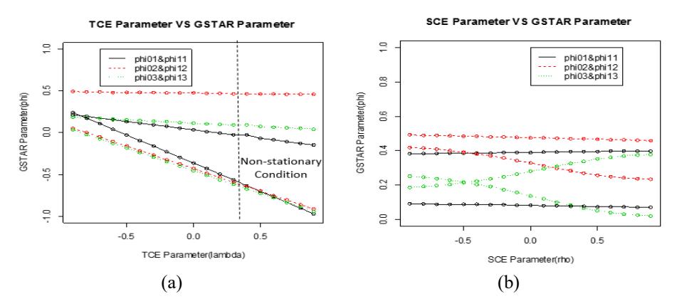
Figure 2 (a) Simulation of temporally correlated errors following a martingale difference process using generalized least squares (Proposition 2). It can be seen that if λ = 0 then the MSE value is the same as with the conventional LS method in Table 1. (b) Simulation of spatially correlated errors using generalized least squares (Proposition 3). If ρ = 0 then the MSE value is the same as with the conventional LS method in Table 1.
5 Case Study
For our case study we used data from the monthly tea production of five plantation sites (N = 5) in West Java, Indonesia (Parakan Salak, Sinumbra,
Rancabali, Rancabolang, and Panyairan) from January 1992 to December 2008 (T = 200). We executed space-time modeling using R Software and started by centering the processes in order to obtain a zero mean.
5.1 Descriptive Statistics
The following data are plot and boxplot data of the monthly tea production from each of the five locations for the period of January 1992 – August 2008.
In Figure 3(a) it can be seen that the production data from Parakan Salak, Rancabali, and Rancabolang have a fairly constant mean but a variance that is not constant. As for the production data from Sinumbra and Panyairan, they are seen trending downward and the variance is not constant. In the box-plot (Figure 3(b)) all the data have outliers, both top and bottom outliers. Maximum and minimum values for each data can be seen in Table 2, while two other locations have only bottom outliers.
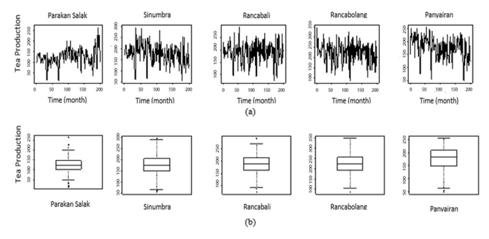
Figure 3 Line-plot (a) and boxplot (b) of the monthly tea production data from five locations from January 1992 – August 2008. In the box-plot all of the data have outliers.
The largest mean production was found in the data from Rancabolang, i.e. 221.80 tons, and the lowest in the data from Parakan Salak, i.e. 123.70 tons (this can be seen in terms of its geographical effect or not). Overall, each location has sufficiently symmetrical data. It can be seen that the mean value and median for each location are not significantly different, except in Panyairan. However, looking more in detail, the median value for any data set is always greater than the mean value. Thus, the data display left skewedness. In other words, each location has a similar tendency in its characteristics, so the GSTAR model can be used to predict future production.
| Statistics | Parakan Salak | Sinumbra | Rancabali | Rancabolang | Panyairan |
|---|---|---|---|---|---|
| Mean | 123.70 | 175.20 | 186.70 | 221.80 | 174.60 |
| Median | 124.40 | 176.70 | 187.40 | 224.70 | 182.00 |
| Q1 | 102.60 | 150.40 | 163.40 | 191.70 | 148.30 |
| Q3 | 145.70 | 205.90 | 213.20 | 255.70 | 209.20 |
| Maximum | 264.70 | 295.90 | 291.10 | 347.80 | 254.50 |
| Minimum | 12.28 | 55.73 | 74.87 | 86.89 | 47.92 |
| Stddev | 38.56 | 44.71 | 40.61 | 47.93 | 42.89 |
| Range | 252.38 | 240.21 | 216.27 | 260.87 | 206.55 |
Table 2 Statistical summary of monthly tea production in five locations from January 1992 to August 2008.
5.2 Model Identification
Model identification was done using the space-time autoregressive function (STACF) and space-time partial autoregressive function (STPACF). From Figure 4 it can be seen that the model was identified only at spatial lags of zero and one, so we can use the GSTAR(1;1) model. GSTAR(1;1) was modeled as follows,
\[\mathbf{Y}(t) = (\boldsymbol{\Phi}_{01}\mathbf{I} + \boldsymbol{\Phi}_{11}\mathbf{W})\mathbf{Y}(t-1) + \boldsymbol{\varepsilon}(t-1)\]
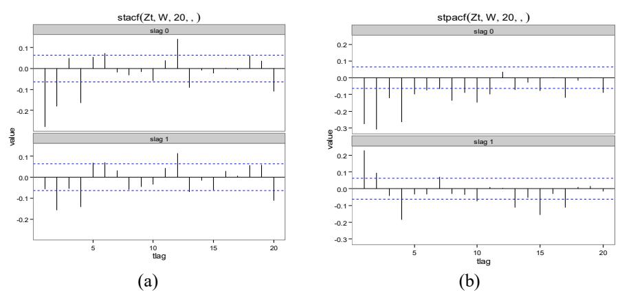
Figure 4 Plot of STACF and STPACF price of chili. The first line is a plot of STACF (a) and STPACF (b) at a spatial lag of zero, while the second line is a plot of STACF (a) and STPACF (b) at a spatial lag of one.
5.3 Parameter Estimation and Diagnostics Test
After identifying the model and obtaining the GSTAR(1;1) model, the next step was to estimate the parameters. But first the weight matrix that characterized the space-time modeling was determined. This study used a uniform weight matrix, which was defined based on the distance between locations. Furthermore, in estimating the GSTAR parameters, the LS method was used, for both the correlated and the uncorrelated error assumptions.
The performances of the GSTAR models for each error assumption were quantitatively compared in terms of root mean square error (RMSE). RMSE is expressed as
\[RMSE = \sqrt{\frac{\sum_{i=1}^{n} (Y_{i} - \hat{Y}_{i})^{2}}{n}}\] where \(Y_i\) and \(\hat{Y}_i\) are the i-th observed and estimated values, respectively; n is the number of validation points.
In this case we used uniform weight matrix \(\mathbf{W}\) to estimate the GSTAR parameters. The uniform weight matrix \(\mathbf{W}\) is
\[\mathbf{W} = \begin{pmatrix} 0 & 0.25 & 0.25 & 0.25 & 0.25 \\ 0.25 & 0 & 0.25 & 0.25 & 0.25 \\ 0.25 & 0.25 & 0 & 0.25 & 0.25 \\ 0.25 & 0.25 & 0.25 & 0 & 0.25 \\ 0.25 & 0.25 & 0.25 & 0.25 & 0 \end{pmatrix}\]
In Section 3.1, performing parameter estimation with the least squares method is described. Using the GSTAR(1;1) model with independent error assumption, the result as shown in Table 3(a) can be obtained.
We also solved GSTAR(1;1) with temporally correlated error assumption. Hence, the GLS method was used to estimate the GSTAR parameters. In this condition, the data errors were assumed to be temporally correlated. The estimation was conducted according to the procedure described in Section 3.2 and the result was as shown in Table 3(b). In the research by Ruhjana et al. [10], parameter estimation of GSTAR(1;1) with temporally correlated error assumption only used the least square method (LS).
In the final simulation, we solved the GSTAR(1;1) model with spatially correlated error assumption. Parameter estimation was conducted using the generalized least squares (GLS) method. This method requires a spatially correlated error (SCE) parameter with values between -1 and 1. By trying some values of \(\rho\), the estimated parameter value in Figure 5 was obtained.
Table 3 Result of parameter estimation using LS for GSTAR(1;1) model with (a) Independent Error Assumption, (b) Temporally Correlated Error Assumption, (c) Spatially Correlated Error Assumption and (d) Seemingly Unrelated Regression.
| lent Error mption | Temporally Correlated Error Assumption | ||||
|---|---|---|---|---|---|
| \(\widehat{\emptyset}_{0}\) | \(\widehat{\emptyset}_{1}\) | \(\widehat{\emptyset}_{0}\) | \(\widehat{\emptyset}_{1}\) | ||
| \[\widehat{\emptyset}_{01} = -0.328\] | \(\widehat{\emptyset}_{11} = 0.030\) | \(\hat{\emptyset}_{01} = -0.33\) | \(\widehat{\emptyset}_{11} = 0.003\) | ||
| \[\widehat{\emptyset}_{02} = -0.386\] | \[\widehat{\emptyset}_{12} = 0.135\] | \(\hat{\emptyset}_{02} = -0.039\) | \(\widehat{\emptyset}_{12} = 0.014\) | ||
| \(\widehat{\emptyset}_{03} = -0.604\) | \(\widehat{\emptyset}_{13} = 0.605\) | \(\hat{\emptyset}_{03} = -0.060\) | \(\widehat{\emptyset}_{13} = 0.061\) | ||
| \(\widehat{\emptyset}_{04} = -0.414\) | \[\widehat{\emptyset}_{14} = 0.600\] | \(\hat{\emptyset}_{04} = -0.041\) | \(\widehat{\emptyset}_{14} = 0.060\) | ||
| \(\hat{\emptyset}_{05} = -0.420\) | \(\widehat{\emptyset}_{15} = 0.116\) | \(\hat{\emptyset}_{05} = -0.042\) | \(\widehat{\emptyset}_{15} = 0.012\) | ||
| (; | a) | (b) | |||
Spatially Correlated Error Assumption
| \(\widehat{\emptyset}_{0}\) | \(\widehat{\emptyset}_1\) |
|---|---|
| \(\hat{\emptyset}_{01} = -0.419\) | \(\widehat{\emptyset}_{11} = 0.080\) |
| \(\widehat{\emptyset}_{02} = -0.417\) | \(\widehat{\emptyset}_{12} = 0.174\) |
| \(\widehat{\emptyset}_{03} = -0.545\) | \(\widehat{\emptyset}_{13} = 0.531\) |
| \(\widehat{\emptyset}_{04} = -0.349\) | \[\widehat{\emptyset}_{14} = 0.522\] |
| \(\widehat{\emptyset}_{05} = -0.441\) | \(\widehat{\emptyset}_{15} = 0.133\) |
| ( | (c) |
GSTAR SUR
| \(\widehat{\emptyset}_{0}\) | \(\widehat{\emptyset}_{1}\) |
|---|---|
| \(\hat{\emptyset}_{01} = -0.412\) | \(\widehat{\emptyset}_{11} = 0.076\) |
| \[\widehat{\emptyset}_{02} = -0.474\] | \[\widehat{\emptyset}_{12} = 0.247\] |
| \(\widehat{\emptyset}_{03} = -0.388\) | \(\widehat{\emptyset}_{13} = 0.332\) |
| \[\widehat{\emptyset}_{04} = -0.558\] | \[\widehat{\emptyset}_{14} = 0.773\] |
| \[\widehat{\emptyset}_{05} = -0.442\] | \(\widehat{\emptyset}_{15} = 0.134\) |
| (d) |
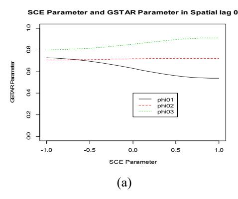
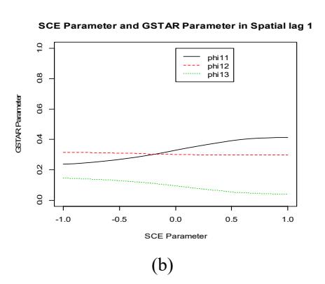
Figure 5 Result of parameter estimation of some SCE parameter values to GSTAR parameters at spatial lag zero (a) and at spatial lag one (b). For all \(\rho \in [-1,1]\) the GSTAR parameters are stationary.
Additional to solving the GSTAR(1;1) problem, with uncorrelated, temporally, and spatially correlated error assumptions using the LS and GLS method, as described in the previous section, we also solved this problem with the SUR method to estimate the model parameters. Treating another problem, Iriany, et al. [9] solved the GSTAR model using the SUR method. We adopted their
technique to solve our data. Hence, the result of solving the GSTAR model could be compared with GLS and SUR. The results show that the SCE method performs better than the SUR method. A plot of each estimation result is shown in Figure 6. In the figure, the red line represents the estimated data and the black line represents the real data. The estimated data plots show similar patterns and are close to the real observations.
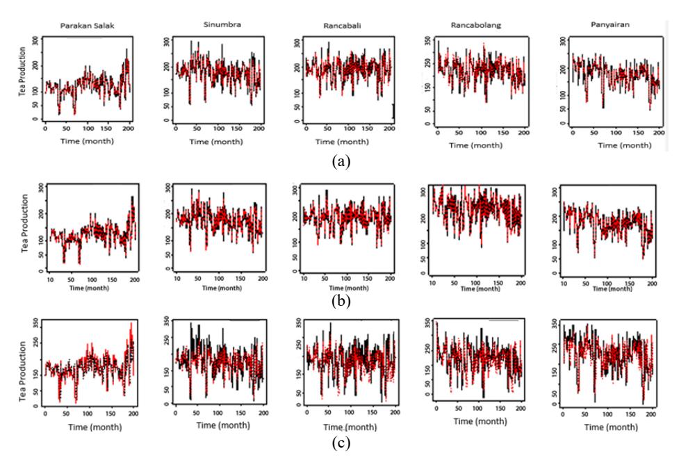
Figure 6 Plots of estimation results using GSTAR(1;1) with (a) independent error, (b) temporally correlated error, (c) spatially correlated error assumption compared with the initial data plot.
Table 4 RMSE Value of GSTAR estimated parameters for each location and each error assumption.
| Model | Parakan Salak | Sinumbra | Rancabali | Rancabolang | Panyairan |
|---|---|---|---|---|---|
| GSTAR(1;1) | 11.28 | 16.68 | 17.85 | 22.38 | 17.60 |
| uncorrelated error | |||||
| GSTAR(1;1) TCE | 1.16 | 1.70 | 5.15 | 9.94 | 7.28 |
| GSTAR(1;1) SCE | 13.93 | 17.47 | 16.34 | 19.79 | 18.23 |
| GSTAR(1;1) SUR | 13.73 | 19.05 | 12.48 | 28.39 | 18.27 |
Note: The smallest RMSE is given by GSTAR (1;1) with temporally correlated error.
The RMSE comparison among independent, temporally, spatially correlated error assumptions, and SUR are shown in Table 4. The smallest RMSE was given by GSTAR(1;1) with temporally correlated error.
In the diagnostic checking stage, we used the correlation error plot at the first lag, the Q-Q normal plot and the histogram, as shown in Figure 7. The correlation error plot at the first lag shows that the errors are random for all methods. The Q-Q normal plot and the histogram show that the normality assumption is satisfied.
Figure 7 Normal probability plot of GSTAR(1;1) errors for each assumption (a) uncorrelated errors, (b) TCE, (c) SCE and (d) SUR.
Table 5 Forecast and errors for four possible error assumptions of GSTAR model.
| Month 201st | |||||||||
|---|---|---|---|---|---|---|---|---|---|
| \(\widehat{Y}_{201}\) | Error | ||||||||
| Uncorrela- ted error | TCE | SCE | SUR | \(Y_{201}\) | Uncorrela- ted error | TCE | SCE | SUR | |
| Parakan Salak | 137.85 | 162.51 | 136.96 | 137.02 | 133.63 | -4.22 | -28.88 | -3.33* | -3.39 |
| Sinumbra | 107.05 | 130.98 | 109.34 | 113.67 | 130.72 | 23.67 | -0.26* | 21.38 | 17.05 |
| Rancabali | 131.82 | 165.22 | 133.30 | 137.26 | 200.98 | 69.16 | 35.76* | 67.68 | 63.72 |
| Rancabolang | 154.50 | 158.06 | 157.32 | 148.24 | 234.75 | 80.25 | 76.69* | 77.43 | 86.51 |
| Panyairan | 116.27 | 146.02 | 116.37 | 116.38 | 100.23 | -16.04* | -45.79 | -16.14 | -16.15 |
Note: The smallest RMSE is given by GSTAR(1;1) with temporally correlated error assumption.
For the forecasting stage, the latest available data were prepared, i.e. the 201<sup>st</sup> month. This forecast observation was compared with real observation. Along with the RMSE result in Table 4, the forecasting result in Table 5 shows that the temporally correlated error assumption still gives the best result, which is shown by the most least errors obtained. The tea production forecast for the next month, i.e. September 2008, at each location (for all assumption used) can be seen in Table 5.
6 Conclusion
Based on the simulation results of the GSTAR model with temporally or spatially correlated error assumption, it can be concluded that the generalized least squares (GLS) method performs better than the conventional least squares method. GLS has an error parameter that can be used as a controller of the model. Hence, it produces an efficient estimator. Hence, this method was applied to real data of monthly tea production. The RMSE value for all methods was obtained (see Table 4). The best model was given by GSTAR(1;1) with temporally correlated assumption. In future studies, different SCE parameter values for each location will be used. The estimation of the model parameters will be tested using the maximum likelihood method for unknown SCE parameter values.
Acknowledgements
We would like to thank Program Riset dan Inovasi ITB 2016 for funding this research.