
1 Introduction
OECD [2] defines time-series data as a set of regular time-ordered observations of a quantitative characteristic from individual or collective phenomena taken at successive and equidistant periods of time. Basically, there are two types of time series, i.e. continuous ones and discrete ones. However, in many subjects, the latter are more easily found and used than the first [3].
To get a better understanding of time-series data characteristics, many researches have been done. Different time-series analysis methods have been developed by esteemed researchers with the final aim of getting a pattern that can be used to predict future values [4]. One of the most widely known methods is the Holt-Winters method. The Holt-Winters method is one of the most commonly used methods from the exponential smoothing family of forecasting methods. It is popular due to its simplicity, low data-storage requirements, and can be easily automated [5]. Two of the most used variations of the Holt-Winters method are the Holt-Winters additive method and the Holt-Winters
multiplicative method [6]. Both of them can be used for predicting time-series data where a trend and seasonal pattern is detected.
In [7], Bermudez, et al. state: "Forecasting competitions have reported the surprising forecasting accuracy of Holt-Winters methods which were obtained with minimal effort in computation and model identification." However, standard exponential smoothing methods are commonly fitted in two steps. The first step is choosing the fixed initial values and the second step is an independent search for parameters [8]. Vercher, et al. [1] have analyzed the importance of choosing proper initial conditions, which results in less forecast errors and better prediction intervals in exponential smoothing models. Accurate estimates of initial conditions can result in better forecasting accuracy [1]. Recently, some researches have proposed maximum likelihood estimation for estimation of smoothing parameters and starting values [9,10], as well as other optimization methods [7,11,12]. In this research, new heuristic rules to estimate initial conditions for the Holt-Winters multiplicative method are introduced. This was motivated by prior researches by Hansun, et al. [13-15], where the basic principle is found in the weighted moving average to give more weight to more recent data, which are then used to estimate the initial values for overall and trend smoothing with the original Holt-Winters multiplicative method.
This paper is composed as follows. The original Holt-Winters multiplicative method as a building block method used in this research is described in Section 2, followed by an explanation of the proposed estimation rules in Section 3. Section 4 is devoted to an explanation of two forecast error measurement criteria, i.e. mean absolute percentage error and mean absolute scaled error. Both of them were used to calculate the accuracy level of the proposed estimation model. Experimental results from 10 different datasets from the United States Census Bureau are shown and discussed in Section 5. Lastly, the paper ends with some concluding remarks.
2 Holt-Winters Multiplicative Method
In the Holt-Winters multiplicative method, the seasonal component is expressed in relative terms and used to adjust the time series seasonally. The multiplicative method can be written in component form as [6]:
\[S_t = \alpha \frac{y_t}{I_{t-L}} + (1 - \alpha)(S_{t-1} + b_{t-1})\] (1)
\[b_t = \gamma (S_t - S_{t-1}) + (1 - \gamma)b_{t-1}\] (2)
\[I_t = \beta \frac{y_t}{(S_{t-1} + b_{t-1})} + (1 - \beta)I_{t-L}\] (3)
where \(S_t\) is the overall smoothing, \(b_t\) is the trend smoothing, and \(I_t\) is the seasonal smoothing. \(y_t\) refers to the real data at time period t. L is the season length, i.e. the number of data points that indicate the beginning of a new season. \(\alpha, \beta\), and \(\gamma\) are constants between 0 to 1, which must be estimated in such a way that the MSE of the error is minimized [16]. Using all three components above, the forecasted value for m periods ahead can be found by using the following formula [6]:
\[F_{t+m} = (S_t + mb_t)I_{t-L+m} \tag{4}\]
As stated by NIST [16], the initial value for the overall smoothing (S) can be taken from the last observation data, while the initial value for trend smoothing can be found by:
\[b = \frac{1}{L} \left( \frac{y_{L+1} - y_1}{L} + \frac{y_{L+2} - y_2}{L} + \dots + \frac{y_{L+L} - y_L}{L} \right)\] (5)
The initial values for the seasonal indices (I) can be computed by calculating the average level for each observed season we have. Then we divide every observed value by the average for the season it is in, and in the final phase we average each number we get across the observed seasons [16,17].
3 The Proposed Estimation Rules
New estimation rules for finding initial conditions for the Holt-Winters multiplicative method are proposed in this paper. We used the basic principle of weighted moving average to give more weight to more recent data and estimate the initial values for the overall smoothing (S) and the trend smoothing (b) components as follows:
\[S = \frac{Ly_L + (L-1)y_{(L-1)} + \dots + (L-m+2)y_{(L-m+2)} + (L-m+1)y_{(L-m+1)}}{L + (L-1) + \dots + (L-m+2) + (L-m+1)}\](6)
\[b = \frac{1}{L^2} \begin{pmatrix} \frac{2Ly_{2L} + (2L-1)y_{(2L-1)} + \dots + (L+2)y_{(L+2)} + (L+1)y_{(L+1)}}{2L + (2L-1) + \dots + (L+2) + (L+1)} \\ -\frac{Ly_L + (L-1)y_{(L-1)} + \dots + 2y_2 + y_1}{L + (L-1) + \dots + 2 + 1} \end{pmatrix}\](7)
where L is season length, m is the span period used for the forecasting, and y are the real data. The initial values for the seasonal indices (I) can be found using the same procedures as in the Holt-Winters multiplicative method. Using all the initial values found, we continue the calculation to find the overall smoothing, trend smoothing, and seasonal smoothing using Eqs. (1-3). Lastly, the forecasted value for m span periods ahead can be found using Eq. (4).
4 Forecast Error Measurement
As stated by Shcherbakov, et al. [18], forecast error measurement can be used to estimate the quality of forecasting methods and to choose the best forecasting mechanism. There are many forecast error measurements, but we will use only two widely known scale-independent error measurements, i.e. mean absolute percentage error and mean absolute scaled error.
4.1 Mean Absolute Percentage Error
Mean absolute percentage error (MAPE) is the average of the absolute error from forecasting results compared to the actual data, which is denoted in percentage form. MAPE is a unit-free error measurement tool, since it expresses the forecasting errors from different measurement units in the form of percentage errors of actual observations [19]. MAPE can be calculated using the following formula [20]:
\[MAPE = \frac{\sum_{t=1}^{n} \left| \frac{e_t}{Y_t} \right|}{n} \times 100 \tag{8}\] where n refers to the number of time-series data and \(e_t\) refers to the forecasting error, which can be expressed as \(Y_t - \hat{Y}_t\).
4.2 Mean Absolute Scaled Error
Mean absolute scaled error (MASE) was first introduced by Hyndman and Koehler [21] as a generally applicable measurement of forecast accuracy on several series with different measurement units. They proposed to scale the forecast errors based on the in-sample mean absolute error (MAE), which is derived from the naïve forecast method [22]. MASE can simply be found using the following formula [21,22]:
\[MASE = mean(|q_t|) \tag{9}\] where \(q_t\) is a scaled error defined as follows [21,22]:
\[q_t = \frac{e_t}{\rho} \tag{10}\] where \(e_t\) denotes the forecasting error from \(Y_t - \hat{Y}_t\), while Q refers to a stable scale's measure of time series calculated on the training data. As explained by Hyndman and Athanasopoulos [6]:
\[Q = \frac{1}{n-1} \sum_{i=2}^{n} |Y_i - Y_{i-1}| \tag{11}\] for non-seasonal time series, and
\[Q = \frac{1}{n-m} \sum_{i=m+1}^{n} |Y_i - Y_{i-m}| \tag{12}\] for seasonal time series data, where ݊ refers to the number of data and ݉ refers to season length.
5 Experimental Results
New estimation rules to find the initial values for the overall smoothing (ܵ) and the trend smoothing (ܾ) component of the Holt-Winters multiplicative method have been described in Section 3. To find the accuracy level of the new estimation model, we tried to apply the model to monthly retail sales data with seasonal factors taken from the United States Census Bureau [23]. 10 different dataset were taken, i.e. Motor Vehicle and Parts Dealers (MVPD), Furniture and Home Furnishings Stores (FHFS), Building Material and Garden Equipment and Supplies Dealers (BMGESD), Grocery Stores (GroS), Gasoline Stations (GaS), Sporting Goods, Hobby, Book, and Music Stores (SGHBMS), Nonstore Retailers (NR), Electronics and Appliance Stores (EAS), Food and Beverage Stores (FBS), and Health and Personal Care Stores (HPCS). The data taken were recorded from January 2011 to December 2015.
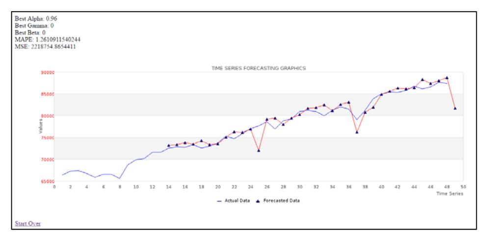
Figure 1 Forecasting results using the Holt-Winters multiplicative method.
The original Holt-Winters multiplicative method and the modified approach for the initial conditions were both tested on all datasets. We used 12 seasonal lengths for both models, with 4 time span periods for the proposed model. As graphed in Figure 1, the forecasting results for the Holt-Winters multiplicative method can be seen, while the forecasting results for the proposed estimation model can be seen in Figure 2. In both figures, a blue line denotes the actual data while a red line denotes the forecasted data.
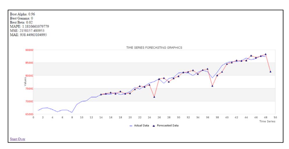
Figure 2 Forecasting results using the proposed estimation model.
All datasets were divided into two subsets. The first subset was used as the training set, while the second subset was used as the testing set, with a 5:1 ratio. The training set is used to get the best parameters that fit the given dataset, while the testing set is used to calculate the accuracy level. For each dataset, we calculated the accuracy level by using MAPE and MASE as described in Section 4. Table 1 shows the best ߙ, ߚ, and ߛ values for each dataset together with the in-sample MAE, which were derived from the naïve forecast method.
| Table 1 | Best Parameter Values for Each Dataset (Training Set). |
|---|
| Dataset | Best α | Best γ | Best β | in-sample MAE-naïve |
|---|---|---|---|---|
| MVPD | 0.96 | 0 | 0.02 | 5755.44 |
| FHFS | 0.64 | 0.02 | 0 | 341.86 |
| BMGESD | 1 | 0 | 0.02 | 1357.64 |
| GroS | 0.94 | 0.02 | 0.12 | 1455.97 |
| GaS | 1 | 0 | 0 | 1696.47 |
| SGHBMS | 0.84 | 0.02 | 0 | 194.69 |
| NR | 0.92 | 0 | 0.02 | 2520.97 |
| EAS | 0.74 | 0 | 0 | 190.28 |
| FBS | 0.86 | 0.02 | 0.12 | 1693.17 |
| HPCS | 1 | 0.02 | 0.14 | 817 |
The accuracy values for each forecasting method implementation on each dataset calculated using MAPE and MASE are shown in Table 2. As can be seen from Table 2, the proposed model has smaller MAPE and MASE values than the original Holt-Winters multiplicative method. Therefore, it has a better accuracy level compared to the Holt-Winters multiplicative method with 27.97% MAPE improvement and 25% MASE improvement compared to the Holt-Winters multiplicative method.
| Table 2 | MAPE and MASE Values of Each Method for 10 Datasets (Testing Set). |
|---|
| Multiplicative HW | Proposed Model | ||||
|---|---|---|---|---|---|
| Dataset | MAPE | MASE | MAPE | MASE | |
| MVPD | 0.8331 | 0.1298 | 0.5891 | 0.0915 | |
| FHFS | 0.9071 | 0.232 | 0.5622 | 0.1442 | |
| BMGESD | 1.0925 | 0.2239 | 0.9891 | 0.2037 | |
| GroS | 0.3851 | 0.1361 | 0.2443 | 0.0864 | |
| GaS | 2.5403 | 0.5378 | 1.3622 | 0.2872 | |
| SGHBMS | 0.8937 | 0.346 | 0.7889 | 0.3062 | |
| NR | 0.7884 | 0.1303 | 0.5971 | 0.0987 | |
| EAS | 1.1783 | 0.5393 | 1.121 | 0.5134 | |
| FBS | 0.4084 | 0.1389 | 0.2588 | 0.088 | |
| HPCS | 0.5854 | 0.1859 | 0.4115 | 0.1308 | |
| Average | 0.96123 | 0.26 | 0.69242 | 0.19501 | |
6 Conclusion
A novel approach to estimate the initial conditions of the Holt-Winters multiplicative method was introduced in this paper. The estimation rules are used to find the initial values for the overall smoothing and the trend smoothing component of the Holt-Winters multiplicative method and are fairly easy to implement.
Based on the experimental results for 10 different datasets from the United States Census Bureau, we found that the proposed estimation model has a better accuracy level, with 27.97% MAPE and 25.00% MASE improvement compared to the original Holt-Winters multiplicative method. Therefore, it is feasible to use as an estimation model for finding initial conditions for the Holt-Winters multiplicative method.
7 Future Works
In a sequel study, implementation of the proposed estimation model to other variants of exponential smoothing methods can be done. A more comprehensive study to develop the model by combining the Holt-Winters method with weighted moving average can also be done. We would like to develop other variations on the hybrid triple exponential smoothing method, for example by using weighted moving average (WMA) combined with Holt-Winters damped method and then analyze its robustness and accuracy levels, etc.
Acknowledgements
The author wishes to thank all fellow researchers at the Multimedia Intelligent System (MIS) Research Group for their support and help.