
1 Introduction
Acceptance sampling plans are used to determine the acceptability of a product unit, where the consumer can accept or reject a lot based on a random sample selected from the lot. The process starts by obtaining the minimum sample size necessary to ascertain a certain average life when the life test is terminated at a predetermined time. Such tests are called truncated life tests. Nowadays acceptance sampling plans are an important tool in quality control because they can help manufacturers to minimize variability and safeguard the outgoing quality of their products.
The concept of an acceptance sampling plan based on truncated life tests has been studied by several authors. For example, Sobel and Tischendrof [1] considered a life test based on an exponential distribution, Gompertz distribution was investigated by Gui and Zhang [2]; Al-Omari [3] studied a three-parameter kappa distribution; Al-Nasser and Al-Omari [4] proposed an acceptance sampling plan based on truncated life tests for the exponentiated Fréchet distribution; Kantam, et al. [5] considered truncated life tests for a loglogistic distribution; Al-Omari [6] considered time truncated acceptance sampling plans using a generalized inverted exponential distribution; Al-Omari [7] proposed transmuted inverse Rayleigh distribution; Aslam and Shabaz [8] considered reliability test plans for a generalized exponential distribution; Al-
Omari [9] studied the generalized inverse Weibull distribution in acceptance sampling plans; Al-Omari, et al. [10] investigated double acceptance sampling plans based on exponentiated generalized inverse Rayleigh distribution; Al-Omari & Zamanzade [11] suggested double acceptance sampling plans for the transmuted generalized inverse Weibull distribution.
The main object of this paper is to present a new acceptance sampling plan based on truncated life tests following a Sushila distribution. This paper is organized as follows. Section 2 delivers the probability density and distribution functions of the Sushila distribution with other statistical properties. Section 3 is devoted to the proposed acceptance sampling plan based on a Sushila distribution and its properties such as the minimum sample size, the operating characteristic function, and the producer's risk. Some useful tables and examples are presented in Section 4. Application of a real data set is given in Section 5. The main conclusions are reported in Section 6.
2 Sushila Distribution
Shanker, et al. [12] suggested a two-parameter (\(\eta\) and \(\delta\)) continuous distribution known as a Sushila distribution (SD), with the probability density function (pdf) defined as:
\[f(x;\eta,\delta) = \frac{\delta^2}{\eta(\delta+1)} \left(1 + \frac{x}{\eta}\right) e^{-\frac{\delta}{\eta}}; \quad x > 0, \delta > 0, \eta > 0.\] (1)
The pdf of the Sushila distribution are shown in Figures 1 for some values of the distribution parameters.
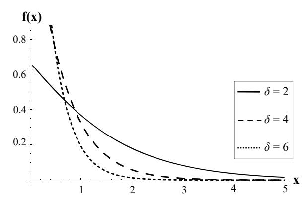
Figure 1 The pdf of the SD with \(\eta = 2\) and \(\delta = 2,4,6\).
The cumulative distribution function (cdf) of the SD random variable is given by:
\[F(x;\eta,\delta) = 1 - \frac{\eta(\delta+1) + \delta x}{\eta(\delta+1)} e^{-\frac{\delta}{\eta}x}, \quad x > 0, \eta > 0, \delta > 0.\] (2)
The cdf of the Sushila distribution are shown in Figures 2 for some values of the distribution parameters.
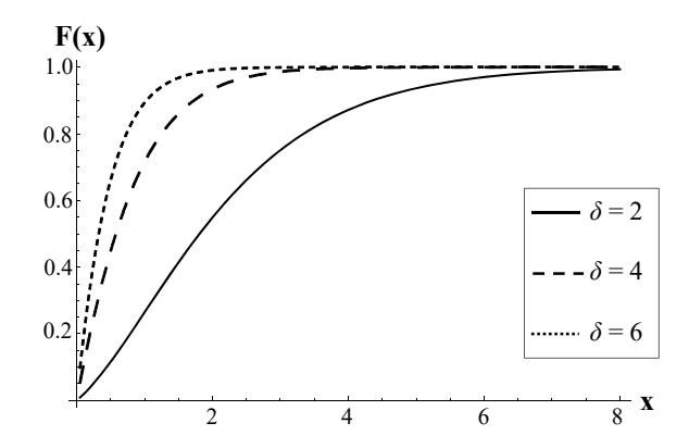
Figure 2 The cdf of the SD with \(\eta = 2\) and \(\delta = 2, 4, 6\).
Shanker, et al. [12] suggested the following properties of the Sushila distribution. The kth moment about the origin of the Sushila random variable can be calculated as follows:
\[\mu'_{k} = E(X^{k}) = k! \left(\frac{\eta + k + 1}{\eta + 1}\right) \left(\frac{\eta}{\delta}\right)^{k}; \quad k = 1, 2, 3, ...\] (3)
Therefore, the first and second moments are:
\[\mu'_1 = E(X) = \frac{\eta + 2}{\eta + 1} \left(\frac{\eta}{\delta}\right) \text{ and } \mu'_2 = E(X^2) = 2\frac{\eta + 3}{\eta + 1} \left(\frac{\eta}{\delta}\right)^2,\] and then the variance of the SD is:
\[\sigma_X^2 = Var(X) = \left(\frac{\eta}{\delta}\right)^2 \left[2\left(\frac{\eta+3}{\eta+1}\right) - \left(\frac{\eta+2}{\eta+1}\right)^2\right]. \tag{4}\]
The mode of the SD is defined as \(Mode = \frac{\eta(1-\delta)}{\delta}\) for \(0 < \delta < 1\), and zero otherwise. The kurtosis \((\varphi)\), skewness (sk) and the coefficient of variation (CV) of the SD, respectively, are given by:
\[\varphi = \frac{3(3\delta^4 + 24\delta^3 + 44\delta^2 + 32\delta + 8)}{(\delta^2 + 4\delta + 2)^2},\] (5)
\[Sk = \frac{2(\delta^{3} + 6\delta^{2} + 6\delta + 2)}{\sqrt{(\delta^{2} + 4\delta + 2)^{3}}},\] (6)
\[CV = \frac{\sqrt{\delta^2 + 4\delta + 2}}{\delta + 2} \,. \tag{7}\]
Note that the measures \(\varphi\), Sk and CV are free of the parameter \(\eta\). The hazard rate function h(x) and mean residual life function m(x) of the Sushila random variable are:
\[h(x) = \frac{\delta^2 (\eta + x)}{\eta [\eta(\delta + 1) + \delta x]},\] (8)
and
\[m(x) = \frac{\eta \left[ \eta(\delta + 1) + \delta x + \eta \right]}{\delta \left[ \eta(\delta + 1) + \delta x \right]}.\] (9)
The method of moment estimate of \(\eta\) is \(\hat{\eta} = \hat{\delta} \overline{X} \left( \frac{\hat{\delta} + 1}{\hat{\delta} + 2} \right)\). For more details about the SD, see Shanker, et al in [12].
3 Suggested Acceptance Sampling Plans
In this section, we propose acceptance sampling plans assuming that the lifetime distribution follows the SD distribution given in Section 2. An acceptance sampling plan based on a Sushila distribution has not been studied before. Also, without loss of generality we assumed that the two parameters \(\eta\) and \(\delta\) are both equal to 2.
An acceptance sampling plan based on truncated life tests consists of the following quantities:
- 1. The number of units (m) on test.
- 2. An acceptance number (c), where if c or less failures happened within the test time (t), the lot is accepted.
- 3. The maximum test duration time, t.
- 4. The ratio \(t/\mu_0\), where \(\mu_0\) is the specified average life.
3.1 Minimum Sample Size
Assume that the lot size is sufficiently large to be considered infinite to obtain the probability of accepting a lot using a binomial distribution. Here, the problem is to determine the smallest sample size m necessary to satisfy the inequality
\[\sum_{i=0}^{c} {m \choose i} p^{i} (1-p)^{m-i} \le 1 - P^{*}, \tag{10}\]
up to an acceptance number c for given values of \(P^* \in (0,1)\), where \(p = F(t; \mu_0)\) is the probability of a failure observed within the time t, which depends only on the ratio \(t/\mu_0\). If the number of observed failures within the time t is at most c, then from Ineq. (10) we can confirm with probability P that \(F(t; \mu) \le F(t; \mu_0)\), which implies \(\mu_0 \le \mu\). The smallest sample sizes that satisfying the Ineq. (9) for \(t/\mu_0 = 0.628, 0.942, 1.257, 1.571, 2.356, 3.141, 3.927, 4.712, <math>P^* = 0.75, 0.9, 0.95, 0.99\) and c = 0,1,2,...,10 are presented in Table 2. The values of \(t/\mu_0\) and \(P^*\) considered in this study are the same values as given in Baklizi, et al. [13], Kantam, et al. [5] and Gupta and Groll [14].
3.2 Operating Characteristic of Sampling Plan \((m, c, t/\mu_0)\)
The operating characteristic (OC) function of sampling plan \((m, c, t/\mu_0)\) provides the probability of acceptance of the lot and is defined as:
\[OC(p) = \sum_{i=0}^{c} {m \choose i} p^{i} (1-p)^{m-i} = 1 - B_{p}(c+1, m-c),\] (11)
where \(p = F(t; \mu)\) is considered to be a function of \(\mu\) (the lot quality parameter), and \(I_p(c+1, m-c)\) is the incomplete beta function defined as:
\[I_g(a,b) = \frac{1}{B(a,b)} \int_0^g \omega^{a-1} (1-\omega)^{b-1} d\omega\], where \(B(a,b) = \frac{(a-1)!(b-1)!}{(a+b-1)!}\) for a, b > 0. The OC function values as a function of \(\mu \ge \mu_0\) for sampling plan \((m, c = 2, t/\mu_0)\) when \(\eta = \delta = 2\) in the SD, as offered in Table 2. Note that for a fixed time, t, OC(p) is a decreasing function of p, while p itself is a monotonically decreasing function of \(\mu \ge \mu_0\). The OC function can be seen as a source for choosing the minimum sample size (m) or the acceptance number (c).
3.3 Producer's Risk
The producer's risk (PR) is defined as the probability of rejecting the lot when \(\mu \ge \mu_0\), and is given by:
\[PR(p) = \sum_{i=c+1}^{m} {m \choose i} p^{i} (1-p)^{m-i} = I_{p}(c+1, m-c).\] (12)
For a given value of the producer's risk, say \(\lambda\), under a given sampling plan, one may be interested in knowing what is the smallest value of \(\mu/\mu_0\) is that will assert a PR of at most \(\lambda\). The value of \(\mu/\mu_0\) is the minimum positive number for which \(p = F\left(\frac{t}{\mu_0}\frac{\mu_0}{\mu}\right)\) satisfies the inequality
\[PR(p) = \sum_{i=c+1}^{m} {m \choose i} p^{i} (1-p)^{m-i} \le \lambda.\] (13)
For a given acceptance sampling plan \((m, c, t/\mu_0)\), at a given confidence level \(P^*\), the smallest values of \(\mu/\mu_0\) satisfying Ineq. (13) are presented in Table 4.
4 Tables and Examples
Table 1 contains the operating characteristic values for sampling plan \((m,c,t/\mu_0)=(8,2,0.942)\) for Table 2. This implies that if the true mean life is twice the specified mean life \((\mu/\mu_0=2)\), the consumer's risk is about 0.583437, while the producer's risk is about 0.1882, 0.077671, 0.03875, 0.021952, 0.013593 for \(\mu/\mu_0=4,6,8,10,12\), respectively. However, when the producer's risk approaches zero, the mean life is at least 10000 or \(\mu/\mu_0 \ge 10\).
Table 1 Operating characteristic values for sampling plan (8, 2, 0.942).
| \(\mu/\mu_0\) | 2 | 4 | 6 | 8 | 10 | 12 |
|---|---|---|---|---|---|---|
| OC | 0. 416563 | 0.811800 | 0. 922329 | 0. 961250 | 0. 978048 | 0. 986407 |
In Table 2, we present the smallest sample sizes necessary to ascertain that the mean life exceeds \(\mu_0\) with probability greater than or equal to \(P^*\), as well as the acceptance number c for \(\eta = \delta = 2\) in the SD distribution. For example, suppose that we want to establish a mean life greater than or equal to least 1000 hours with probability \(P^* = 0.90\). The life test is at least t = 942 hours \((t/\mu_0 = 0.942)\) when the acceptance number c = 2. Then, the corresponding table value is m = 8 units that should be put on test. That is, if within 1000 hours at most 2 units out of 8 units fail before time t, then the lot is accepted. Otherwise it is rejected with a confidence level of 0.90. Thus, the time test has to be truncated at time 0.942 of the specified mean life so that the average life is at least 1000 hours. The sample sizes given in Table 2 are smaller than the sample sizes provided in Baklizi, \(et\ al.\ [13]\), Kantam, \(et\ al.\ [5]\) and Gupta and Groll [14].
Table 3 shows the operating characteristic function (OC) values for the time truncated acceptance sampling plan calculated from Table 2 for various values of \(t/\mu_0\) and \(P^*\) with acceptance number c=2. Operating characteristic values for sampling plan.
Table 2 Minimum sample sizes necessary to ensure mean life to exceed given value ߤ with probability ܲ∗ and acceptance number c for a SD with η = δ = 2.
| ࣆ/ࣆ ࢉ | |||||||||
|---|---|---|---|---|---|---|---|---|---|
| ∗ࡼ | 0.628 | 0.942 | 1.257 | 1.571 | 2.356 | 3.141 | 3.927 | 4.712 | |
| 0.75 | 0 | 3 | 2 | 2 | 1 | 1 | 1 | 1 | 1 |
| 1 | 6 | 4 | 3 | 3 | 2 | 2 | 2 | 2 | |
| 2 | 8 | 6 | 5 | 4 | 3 | 3 | 3 | 3 | |
| 3 | 11 | 8 | 6 | 6 | 5 | 4 | 4 | 4 | |
| 4 | 13 | 10 | 8 | 7 | 6 | 5 | 5 | 5 | |
| 5 6 | 16 18 | 12 13 | 10 11 | 8 10 | 7 8 | 6 7 | 6 7 | 6 7 | |
| 7 | 21 | 15 | 13 | 11 | 9 | 9 | 8 | 8 | |
| 8 | 23 | 17 | 14 | 12 | 10 | 10 | 9 | 9 | |
| 9 | 26 | 19 | 16 | 14 | 12 | 11 | 10 | 10 | |
| 10 | 28 | 21 | 17 | 15 | 13 | 12 | 11 | 11 | |
| 0.90 | 0 | 4 | 3 | 2 | 2 | 1 | 1 | 1 | 1 |
| 1 | 8 | 5 | 4 | 4 | 3 | 2 | 2 | 2 | |
| 2 | 11 | 8 | 6 | 5 | 4 | 4 | 3 | 3 | |
| 3 | 13 | 10 | 8 | 7 | 5 | 5 | 4 | 4 | |
| 4 | 16 | 12 | 9 | 8 | 6 | 6 | 5 | 5 | |
| 5 | 19 | 14 | 11 | 9 | 8 | 7 | 6 | 6 | |
| 6 | 22 | 16 | 13 | 11 | 9 | 8 | 7 | 7 | |
| 7 | 24 | 17 | 14 | 12 | 10 | 9 | 9 | 8 | |
| 8 | 27 | 19 | 16 | 14 | 11 | 10 | 10 | 9 | |
| 9 | 29 | 21 | 17 | 15 | 12 | 11 | 11 | 10 | |
| 10 | 32 | 23 | 19 | 16 | 14 | 12 | 12 | 11 | |
| 0.95 | 0 | 6 | 4 | 3 | 2 | 2 | 1 | 1 | 1 |
| 1 2 | 9 12 | 6 9 | 5 7 | 4 6 | 3 4 | 3 4 | 2 3 | 2 3 | |
| 3 | 15 | 11 | 9 | 7 | 6 | 5 | 5 | 4 | |
| 4 | 18 | 13 | 10 | 9 | 7 | 6 | 6 | 5 | |
| 5 | 21 | 15 | 12 | 10 | 8 | 7 | 7 | 6 | |
| 6 | 24 | 17 | 14 | 12 | 9 | 8 | 8 | 7 | |
| 7 | 27 | 19 | 15 | 13 | 11 | 9 | 9 | 8 | |
| 8 | 29 | 21 | 17 | 15 | 12 | 10 | 10 | 10 | |
| 9 | 32 | 23 | 19 | 16 | 13 | 12 | 11 | 11 | |
| 10 | 35 | 25 | 20 | 17 | 14 | 13 | 12 | 12 | |
| 0.99 | 0 | 8 | 6 | 4 | 3 | 2 | 2 | 2 | 1 |
| 1 | 12 | 8 | 6 | 5 | 4 | 3 | 3 | 3 | |
| 2 | 16 | 11 | 8 | 7 | 5 | 4 | 4 | 4 | |
| 3 | 19 | 13 | 10 | 9 | 7 | 6 | 5 | 5 | |
| 4 | 22 | 16 | 12 | 10 | 8 | 7 | 6 | 6 | |
| 5 | 25 | 18 | 14 | 12 | 9 | 8 | 7 | 7 | |
| 6 | 28 | 20 | 16 | 13 | 10 | 9 | 8 | 8 | |
| 7 | 31 | 22 | 18 | 15 | 12 | 10 | 9 | 9 | |
| 8 | 34 | 24 | 19 | 16 | 13 | 11 | 10 | 10 | |
| 9 | 37 | 26 | 21 | 18 | 14 | 12 | 12 | 11 | |
| 10 | 40 | 28 | 23 | 19 | 15 | 14 | 13 | 12 | |
Table 3 Operating characteristic values for sampling plan ሺ݊, ܿ, ݐ/ߤ (for given probability ܲ∗ with acceptance number ܿൌ2 for a SD with η = δ = 2.
| ∗ࡼ | ||||||||
|---|---|---|---|---|---|---|---|---|
| ࣆ/࢚ | 2 | 4 | 6 | 8 | 10 | 12 | ||
| 0.75 | 9 | 0.628 | 0.677562 | 0.922329 | 0.971212 | 0.986407 | 0.992553 | 0.995491 |
| 6 | 0.942 | 0.637505 | 0.909354 | 0.966006 | 0.983859 | 0.991128 | 0.994617 | |
| 5 | 1.257 | 0.599288 | 0.895882 | 0.960470 | 0.981121 | 0.989588 | 0.993668 | |
| 4 | 1.571 | 0.646544 | 0.912949 | 0.967631 | 0.984711 | 0.991626 | 0.994932 | |
| 3 | 2.356 | 0.681263 | 0.923378 | 0.971815 | 0.986772 | 0.992786 | 0.995647 | |
| 3 | 3.141 | 0.505867 | 0.854051 | 0.942157 | 0.971823 | 0.984288 | 0.990380 | |
| 3 | 3.927 | 0.356962 | 0.770811 | 0.902244 | 0.950563 | 0.971809 | 0.982482 | |
| 3 | 4.712 | 0.243265 | 0.681263 | 0.854018 | 0.923378 | 0.955314 | 0.971815 | |
| 0.90 | 11 | 0.628 | 0.453982 | 0.830181 | 0.930753 | 0.965650 | 0.980605 | 0.988016 |
| 8 | 0.942 | 0.416563 | 0.811800 | 0.922329 | 0.961250 | 0.978048 | 0.986407 | |
| 6 | 1.257 | 0.448315 | 0.829663 | 0.931016 | 0.965938 | 0.980829 | 0.988183 | |
| 5 | 1.571 | 0.450179 | 0.831074 | 0.931826 | 0.966416 | 0.981129 | 0.988381 | |
| 4 | 2.356 | 0.378229 | 0.791143 | 0.912992 | 0.956475 | 0.975324 | 0.984720 | |
| 3 | 3.141 | 0.195428 | 0.646731 | 0.835737 | 0.913013 | 0.948957 | 0.967658 | |
| 3 | 3.927 | 0.356962 | 0.770811 | 0.902244 | 0.950563 | 0.971809 | 0.982482 | |
| 3 | 4.712 | 0.243265 | 0.681263 | 0.854018 | 0.923378 | 0.955314 | 0.971815 | |
| 0.95 | 13 | 0.628 | 0.389457 | 0.794630 | 0.913643 | 0.956467 | 0.975176 | 0.984559 |
| 9 | 0.942 | 0.326343 | 0.756132 | 0.894618 | 0.946139 | 0.969032 | 0.980632 | |
| 7 | 1.257 | 0.323003 | 0.755223 | 0.894496 | 0.946181 | 0.969100 | 0.980694 | |
| 6 | 1.571 | 0.295254 | 0.736152 | 0.884847 | 0.940904 | 0.965952 | 0.978680 | |
| 4 | 2.356 | 0.378229 | 0.791143 | 0.912992 | 0.956475 | 0.975324 | 0.984720 | |
| 4 | 3.141 | 0.195428 | 0.646731 | 0.835737 | 0.913013 | 0.948957 | 0.967658 | |
| 3 | 3.927 | 0.356962 | 0.770811 | 0.902244 | 0.950563 | 0.971809 | 0.982482 | |
| 3 | 4.712 | 0.243265 | 0.681263 | 0.854018 | 0.923378 | 0.955314 | 0.971815 | |
| 0.99 | 17 | 0.628 | 0.196131 | 0.642796 | 0.831100 | 0.909359 | 0.946275 | 0.965695 |
| 11 | 0.942 | 0.191124 | 0.640140 | 0.830181 | 0.909025 | 0.946150 | 0.965650 | |
| 9 | 1.257 | 0.225923 | 0.677121 | 0.852234 | 0.922185 | 0.954438 | 0.971154 | |
| 7 | 1.571 | 0.185247 | 0.637107 | 0.829369 | 0.908885 | 0.946201 | 0.965749 | |
| 5 | 2.356 | 0.186160 | 0.639004 | 0.831149 | 0.910210 | 0.947150 | 0.966434 | |
| 4 | 3.141 | 0.195428 | 0.646731 | 0.835737 | 0.913013 | 0.948957 | 0.967658 | |
| 4 | 3.927 | 0.092934 | 0.504016 | 0.744073 | 0.856684 | 0.912975 | 0.943576 | |
| 4 | 4.712 | 0.041834 | 0.378229 | 0.646669 | 0.791143 | 0.868829 | 0.912992 |
Table 4 Minimum ratio of true mean life to specified life for the acceptability of a lot with a producer's risk of 0.05 for a SD with η = δ = 2.
| ࢉ /࢚ ࣆ | |||||||||
|---|---|---|---|---|---|---|---|---|---|
| ∗ࡼ | 0.628 | 0.942 | 1.257 | 1.571 | 2.356 | 3.141 | 3.927 | 4.712 | |
| 0.75 | 0 | 32.758 | 32.791 | 43.757 | 27.426 | 41.130 | 54.835 | 68.556 | 82.260 |
| 1 | 8.677 | 8.261 | 7.821 | 9.775 | 8.516 | 11.353 | 14.194 | 17.032 | |
| 2 | 4.811 | 5.139 | 5.458 | 5.044 | 4.778 | 6.370 | 7.964 | 9.556 | |
| 3 | 3.916 | 4.006 | 3.655 | 4.568 | 5.217 | 4.636 | 5.796 | 6.954 | |
| 4 | 3.150 | 3.425 | 3.396 | 3.495 | 4.080 | 3.765 | 4.708 | 5.649 | |
| 5 | 2.919 | 3.071 | 3.211 | 2.875 | 3.415 | 3.241 | 4.052 | 4.862 | |
| 6 | 2.582 | 2.568 | 2.715 | 2.939 | 2.978 | 2.889 | 3.612 | 4.334 | |
| 7 | 2.489 | 2.440 | 2.669 | 2.582 | 2.669 | 3.558 | 3.295 | 3.954 | |
| 8 | 2.293 | 2.341 | 2.374 | 2.320 | 2.438 | 3.251 | 3.054 | 3.665 | |
| 9 | 2.247 | 2.262 | 2.369 | 2.405 | 2.732 | 3.012 | 2.865 | 3.437 | |
| 10 | 2.115 | 2.196 | 2.167 | 2.215 | 2.541 | 2.820 | 2.711 | 3.253 | |
| 0.9 | 0 | 43.655 | 49.137 | 43.757 | 54.687 | 41.130 | 54.835 | 68.556 | 82.260 |
| 1 | 11.834 | 10.642 | 11.023 | 13.777 | 14.659 | 11.353 | 14.194 | 17.032 | |
| 2 | 6.874 | 7.216 | 6.857 | 6.821 | 7.565 | 10.085 | 7.964 | 9.556 | |
| 3 | 4.741 | 5.254 | 5.346 | 5.631 | 5.217 | 6.955 | 5.796 | 6.954 | |
| 4 | 4.009 | 4.293 | 3.986 | 4.245 | 4.080 | 5.440 | 4.708 | 5.649 | |
| 5 | 3.567 | 3.727 | 3.656 | 3.450 | 4.312 | 4.553 | 4.052 | 4.862 | |
| 6 | 3.271 | 3.354 | 3.426 | 3.393 | 3.709 | 3.970 | 3.612 | 4.334 | |
| 7 | 2.915 | 2.874 | 2.963 | 2.962 | 3.286 | 3.558 | 4.449 | 3.954 | |
| 8 | 2.775 | 2.709 | 2.876 | 2.966 | 2.974 | 3.251 | 4.064 | 3.665 | |
| 9 | 2.561 | 2.581 | 2.587 | 2.685 | 2.732 | 3.012 | 3.765 | 3.437 | |
| 10 | 2.483 | 2.477 | 2.552 | 2.464 | 2.939 | 2.820 | 3.526 | 3.253 | |
| 0.95 | 0 | 65.448 | 65.482 | 65.568 | 54.687 | 82.013 | 54.835 | 68.556 | 82.260 |
| 1 | 13.411 | 13.016 | 14.201 | 13.777 | 14.659 | 19.544 | 14.194 | 17.032 | |
| 2 | 7.560 | 8.249 | 8.246 | 8.570 | 7.565 | 10.085 | 7.964 | 9.556 | |
| 3 | 5.564 | 5.874 | 6.180 | 5.631 | 6.850 | 6.955 | 8.695 | 6.954 | |
| 4 | 4.581 | 4.724 | 4.570 | 4.982 | 5.241 | 5.440 | 6.801 | 5.649 | |
| 5 | 3.999 | 4.053 | 4.097 | 4.013 | 4.312 | 4.553 | 5.692 | 4.862 | |
| 6 | 3.614 | 3.614 | 3.778 | 3.840 | 3.709 | 3.970 | 4.964 | 4.334 | |
| 7 | 3.341 | 3.305 | 3.256 | 3.335 | 3.873 | 3.558 | 4.449 | 3.954 | |
| 8 | 3.016 | 3.075 | 3.124 | 3.282 | 3.479 | 3.251 | 4.064 | 4.876 | |
| 9 | 2.873 | 2.898 | 3.018 | 2.961 | 3.178 | 3.643 | 3.765 | 4.518 | |
| 10 | 2.758 | 2.756 | 2.742 | 2.709 | 2.939 | 3.387 | 3.526 | 4.230 | |
| 0.99 | 0 | 87.241 | 98.172 | 87.378 | 81.946 | 82.013 | 109.338 | 136.699 | 82.260 |
| 1 | 18.136 | 17.751 | 17.368 | 17.748 | 20.661 | 19.544 | 24.434 | 29.318 | |
| 2 | 10.302 | 10.311 | 9.629 | 10.306 | 10.23 | 10.085 | 12.608 | 15.129 | |
| 3 | 7.207 | 7.112 | 7.010 | 7.723 | 8.444 | 9.132 | 8.695 | 10.433 | |
| 4 | 5.721 | 6.014 | 5.728 | 5.712 | 6.365 | 6.987 | 6.801 | 8.160 | |
| 5 | 4.859 | 5.027 | 4.973 | 5.121 | 5.174 | 5.748 | 5.692 | 6.829 | |
| 6 | 4.299 | 4.390 | 4.475 | 4.282 | 4.407 | 4.944 | 4.964 | 5.956 | |
| 7 | 3.906 | 3.947 | 4.123 | 4.069 | 4.442 | 4.381 | 4.449 | 5.338 | |
| 8 | 3.616 | 3.620 | 3.615 | 3.594 | 3.969 | 3.964 | 4.064 | 4.876 | |
| 9 | 3.393 | 3.370 | 3.444 | 3.503 | 3.607 | 3.643 | 4.554 | 4.518 | |
| 10 | 3.215 | 3.173 | 3.305 | 3.189 | 3.321 | 3.918 | 4.234 | 4.230 | |
Table 4 displays the minimum ratio between the true mean lifetime and the specified one for acceptance of the lot with the producer's risk \(\lambda=0.05\). However, we can get the value of \(\mu/\mu_0\) for various choices of c, \(t/\mu_0\) such that the producer's risk may not exceed 0.05. Thus, in our example, the value of \(\mu/\mu_0\) is 7.216 for c=2, \(t/\mu_0=0.942\), and \(P^*=0.90\) or the consumer's risk is 0.10. That is, the lot will be rejected with probability at most 0.05, which implies that the product can have a mean life of 7.216 times the specified average lifetime of 1000 hours in order to accept the product with probability at least 0.95. The actual average lifetime required to accept 95% of the lot is presented in Table 4.
5 Real Data Application
The data given in this section were considered by Lawless [15]. The data are the number of million revolutions before failure for each of 23 ball bearings in a life test. The data values are: 51.84, 51.96, 54.12, 68.88, 55.56, 67.80, 68.44, 68.64, 84.12, 98.64, 105.12, 93.12, 105.84, 127.92, 128.04 and 173.40.
The maximum likelihood estimators of the parameters of the Sushila distribution based on these data are \(\hat{\eta}=0.4780671\) with a standard deviation of 0.65001495 and \(\hat{\delta}=0.0108697\) with a standard deviation of 0.01461223. For the data it was found that the Kolmogorov-Smirnov distance is 0.333551 with p-value 0.04342598, the Cramér-von Mises criterion is W=0.06575653, the Anderson-Darling criterion is A=0.4429015, the Bayesian information criterion is 170.585, the consistent Akaike information criterion is 169.9629, the maximized log-likelihood is 82.51989 and the Hannan-Quinn information criterion is 169.1189. Hence, the Sushila distribution could provide reasonable goodness of fit for the ball bearing data set.
Suppose that the lifetime of a product follows the Sushila distribution and the specified average life is \(\hat{\mu}_0 = \frac{\hat{\eta} + 2}{\hat{\eta} + 1} \left( \frac{\hat{\eta}}{\hat{\delta}} \right) = 80.43\) million revolutions. Assume that the researcher wishes to end the test at \(t_0 = 75.77\) million revolutions, i.e. equivalent to \(t_0/\mu_0 = 0.628\) for acceptance number c = 8. Hence, for confidence level \(P^* = 0.75\), the sampling plan is \((m = 23, c = 8, t/\mu_0 = 0.628)\). If no more than 8 failures out of the 23 ball bearings are observed at the end of time t, then the lot is accepted. Hence, the lot is accepted in this experiment.
6 Conclusions
In this work, a time truncated acceptance sampling plan was developed for truncated life tests following a Sushila distribution. Some useful tables were presented and applied for the minimum sample size necessary to guarantee a certain mean life of the test units, the operating characteristic function values for the sampling plan, and the minimum ratio to the specified mean life for accepting a lot with confirmed producer's risk. Practitioners can use the results obtained in this paper and the proposed method can also be used for other distributions that can be converted to a Sushila distribution.
Acknowledgements
The authors are indebted to the referee and the editors for their helpful suggestions.