
1 Introduction
In this paper we connect, in a general and elementary way, the theory of polynomial meshes with the theory of polynomial optimization. We begin by the definition of polynomial mesh, a notion that has been playing a relevant role in recent research on multivariate polynomial approximation.
We recall that a polynomial mesh of a compact subset K of \(\mathbb{R}^d\) (or more generally of a manifold \(\mathcal{M} \subseteq \mathbb{R}^d\)) is a sequence of finite norming subsets \(\mathcal{A}_n \subset K\) such that the polynomial inequality
\[\|p\|_{K} \le c \|p\|_{\mathcal{A}_{n}}, \forall p \in \mathbb{P}_{n}^{d}(K),\] (1)
holds for some constant c > 1 (independent of p and n but dependent in general on d), where
\[card(\mathcal{A}_n) = \mathcal{O}(N_n^s), \ s \ge 1, \ N_n = N_n(K) = dim(\mathbb{P}_n^d(K)).\] (2)
Here and below we denote by \(\mathbb{P}_n^d(K)\) the subspace of d-variate polynomials of total degree not exceeding n restricted to K. For example, we have that \(N_n = \binom{n+3}{3} = (n+1)(n+2)(n+3)/6\) for the ball in \(\mathbb{R}^3\) and \(N_n = (n+1)^2\) for the sphere \(S^2\).
Observe that n is ℙ ௗሺܭሻ-determining (i.e. a polynomial vanishing there vanishes everywhere on ܭ(, consequently ( ) n n card N ; a polynomial mesh may then be termed optimal when ݏൌ1. All these notions can be given more generally for d K but we restrict here to real compact sets. They are extensions of notions usually given for d .
Among the relevant properties of polynomial meshes we recall that they are affinely invariant, can be extended by finite union and product and by algebraic transformations, are stable under small perturbations, and overall they are near optimal for polynomial least squares, and contain near optimal interpolation subsets (in the sense of the growth rate of the Lebesgue constant); cf. for example [1,2]. Moreover, they are nice discrete models of Bernstein-Markov measures, cf. [3].
As shown in the seminal paper [2], where the notion of the polynomial mesh was originally introduced, uniform meshes are polynomial meshes (on compact sets admitting a Markov polynomial inequality) only for high density (and thus for high cardinality), whereas to get low cardinality we need nonuniform meshes, with a distribution that is related in a deep way to the pluripotential equilibrium measure of the compact set (cf. for example [1,3]).
Optimal polynomial meshes, i.e. polynomial meshes with optimal cardinality growth, namely ( ) ( ) n n card N , have been constructed on various classes of compact sets, such as polygons and polyhedra, sections of a disk, sphere, ball, torus, convex bodies and star-shaped domains, general compact sets with regular boundary; we refer the reader to, for example, [4-7] and the references therein, for a comprehensive view of properties, construction methods and applications.
2 Optimization on Optimal Meshes
Polynomial optimization on uniform grids of standard domains (box, simplex) has been an object of some interest in the last twenty years (cf. for example [8,9] and the references therein), whereas nonuniform grids (of Chebyshev type) together with the corresponding polynomial inequalities have been considered only on multidimensional boxes, for example in [10] and more recently in [11].
On the other hand, the general theory of polynomial meshes (which is ultimately a matter of discrete polynomial inequalities) has not yet entered the framework of continuous optimization. The following proposition estabilishes a possible connection.
Proposition 1. Let \(\{A_n\}\) be a polynomial mesh of a compact set \(K \subset \mathbb{R}^d\). Denote by \(\overline{p} = \max_{x \in K} p(x)\), \(p = \min_{x \in K} p(x)\),
\[\overline{p}_m = \max_{x \in \mathcal{A}_{-}} p(x), \quad p_m = \min_{x \in \mathcal{A}_{-}} p(x), \tag{3}\] the continuous and discrete extrema of \(p \in \mathbb{P}_n^d\), where \(m \in \mathbb{N}\), \(m \ge 2\).
Then, the following estimate holds:
\[\max\{\overline{p} - \overline{p}_m, \underline{p}_m - \underline{p}\} \le E_m(\overline{p} - \underline{p}), \tag{4}\]
\[E_m = \frac{c^{1/m} \log(c)}{m} \sim \frac{\log(c)}{m}, \ m \to \infty.\] (5)
Proof. First, observe that if \(\mathcal{A}_n\) is a polynomial mesh with constant c, then \(\mathcal{A}_{mn}\) is a polynomial mesh with constant \(c^{1/m}\). In fact, if \(p \in \mathbb{P}_n^d\) then \(p^m \in \mathbb{P}_{mn}^d\) and we can write:
\[\parallel p^m \parallel_K = \parallel p \parallel_K^m \le c \parallel p^m \parallel_{\mathcal{A}_{mn}} = c \parallel p \parallel_{\mathcal{A}_{mn}}^m\]
Now consider the polynomial \(q(x) = p(x) - \overline{p} \in \mathbb{P}_n^d\) which is nonpositive in K. We have that \(\|q\|_K = |\underline{p} - \overline{p}| = \overline{p} - \underline{p}\), and \(\|q\|_{A_{mn}} = |\underline{p}_m - \overline{p}| = \overline{p} - \underline{p}_m\). Then by Eq. (1)
\[\underline{p}_{m} - \underline{p} = \|q\|_{K} - \|q\|_{\mathcal{A}_{mn}} \le (c^{1/m} - 1)\|q\|_{\mathcal{A}_{mn}} \le (c^{1/m} - 1)\|q\|_{K} = (c^{1/m} - 1)(\overline{p} - \underline{p}).\]
The other estimate in Eq. (4) is obtained similarly, taking \(q(x) = p(x) - \underline{p}\) which is nonnegative in K.
We conclude by observing that \(c^{1/m} - 1 = e^{\log(c)/m} - 1 \le e^{\log(c)/m} \frac{\log(c)}{m}\) by the mean value theorem and the monotonicity of the exponential function. \(\Box\)
Observe that the error \(E_m\) is relative to the range of p, a usual requirement in polynomial optimization; in particular, we may say that \(\overline{p}_m\) and \(\underline{p}_m\) are \((1 - E_m)\)-approximations to the corresponding polynomial extrema, cf. e.g. [8].
The complexity of the discrete optimization is proportional to the number of evaluations of the polynomial, i.e. to the cardinality of \(\mathcal{A}_{mn}\). If \(\{\mathcal{A}_n\}\) is an optimal mesh then Eq. (2) holds with s=1 and \(card(\mathcal{A}_{mn})=\mathcal{O}(N_{mn})\). We may now distinguish two situations.
The first occurs when K is polynomial determining (i.e. polinomials vanishing there vanish everywhere in \(\mathbb{R}^d\)), for example when K has nonempty interior; in this case \(N_{nm} = \binom{mn+d}{d} \sim (mn)^d/d!\) (for d fixed and \(mn \to \infty\)).
The second occurs when K is a compact subset of a real algebraic variety \(\mathcal{M} \subset \mathbb{R}^d\) (which is determining for polynomials restricted to \(\mathcal{M}\)). In this case \(N_{mn} = \mathcal{O}((mn)^{\beta})\) with \(\beta < d\). For example, if the variety is the zero set of an irreducible real polynomial of degree k, then
\[N_{mn} = dim(\mathbb{P}_{mn}^{d}(K)) = dim(\mathbb{P}_{mn}^{d}(\mathcal{M})) = \binom{mn+d}{d} - \binom{mn-k+d}{d}, \quad (6)\] for \(mn \ge k\), and thus \(N_{mn} \sim \frac{k}{(d-1)!} (mn)^{d-1}\) for \(mn \to \infty\) (d and k fixed). To illustrate this point, we have that the sphere is a quadric (k = 2), whereas the torus is a quartic (k = 4) surface in d = 3 variables, see for example [12] for the relevant algebraic geometry notions.
Now, fix \(\varepsilon \in (0,1]\). Following the usual definitions (cf. for example [8]), to get a \((1 - \varepsilon)\)-approximation scheme from Proposition 1, that is
\[\max\{\overline{p} - \overline{p}_{m}, p_{m} - p\} \le \varepsilon(\overline{p} - p), \tag{7}\]
we should take \(m = m(\varepsilon) = \mathcal{O}\left(\varepsilon^{-1}\right)\), since \(E_m = \mathcal{O}\left(m^{-1}\right)\) (for fixed d), a rough estimate being \(E_m \leq \sqrt{c}\log(c)/m\). Then \(mn = \mathcal{O}\left(\varepsilon^{-1}n\right)\), and by the considerations above \(N_{mn} = \mathcal{O}\left((\varepsilon^{-1}n)^{\beta}\right)\), with \(\beta = d\) (if K is polynomial determining on \(\mathbb{R}^d\)), or \(\beta < d\) (if K is not polynomial determining on \(\mathbb{R}^d\), for example a subset of an algebraic variety).
As recalled in the introduction, optimal polynomial meshes have been constructed on compact sets with different structures, by various geometrical and analytical tools. Some of these constructions are simple and efficient, other require deep analytical results and are difficult to implement.
In order to give an example of a class of compact sets where optimal polynomial meshes are known, we show in Table 1 a number of standard circular sections of disk, sphere and torus, that are obtained by cutting the geometric objects by lines or planes, or by making suitable set intersections or differences. The sections are grouped by the constant ܿ of the corresponding optimal polynomial meshes, whose cardinality is displayed. We do not go here into details of the construction and of the mesh constant estimation, which are based on suitable bilinear trigonometric transformations and 'subperiodic' trigonometric polynomial inequalities (indeed, circular arcs and thus subintervals of the period are involved); cf. for example [7,13,14] with the references therein.
Table 1 Some standard planar, surface and solid circular sections together with the corresponding polynomial mesh parameters.
| ࢉ | mn card ( ) (bound) | Section type | |
|---|---|---|---|
| √2 | 4݉݊ 1 | entire cicle | |
| 2 | 4݉݊ 1 ሺ2݉݊ 1ሻሺ4݉݊ 1ሻ | circle arc entire disk/disk annulus | |
| ሺ4݉݊ 1ሻଶ | entire sphere/torus | ||
| 2√2 | ሺ2݉݊ 1ሻሺ4݉݊ 1ሻ ሺ4݉݊ 1ሻଶ | disk sector/segment/zone/lens surface spherical cap/collar surface toroidal cap/collar/slice | |
| ሺ2݉݊ 1ሻሺ4݉݊ 1ሻଶ | entire ball/solid torus spherical shell | ||
| 4 | ሺ4݉݊ 1ሻଶ | planar lune surface spherical rectangle/lune surface toroidal rectangle | |
| ሺ2݉݊ 1ሻሺ4݉݊ 1ሻଶ | solid spherical cap/cone/lens/zone solid toroidal cap/slice/zone | ||
| 4√2 | ሺ2݉݊ 1ሻሺ4݉݊ 1ሻଶ | spherical square pyramid | |
| 8 | ሺ4݉݊ 1ሻଷ | solid lune | |
To show a specific application, by Proposition 1 and Table 1 we see that one can obtain an approximation of the extremal values of any trivariate polynomial of degree ݊ൌ4 (restricted to a surface spherical or toroidal cap of any angular extension) within about 10% of the polynomial range െ ሺܿ ൌ 2√2, ݉ ൌ 10ሻ, by evaluating the polynomial on the optimal polynomial mesh given by a grid of 161×161 points. By no loss of generality, on the sphere we can take a polar cap. The grids have the form
\[\mathcal{A}_{mn} = \sigma(\Theta_{mn} \times \Phi_{mn}),\] \[\sigma(\theta, \phi) = ((R + r\cos(\theta))\cos(\phi), (R + r\cos(\theta))\sin(\phi), r\sin(\theta)),\] (8)
with ܴൌ0 (sphere) or ܴݎ0) torus),
\[\Phi_{mn} = \{ \phi_j = 2\pi j / (4mn + 2), 1 \le j \le 4mn + 1 \} \subset (0, 2\pi),\] and
\[\Theta_{mn} = \left\{ \theta_i = \frac{\pi}{2} + 2\arcsin(\sin(\omega/2)t_i), \ 0 \le i \le 4mn \right\} \subset \left(\frac{\pi}{2} - \omega, \frac{\pi}{2} + \omega\right),\]
\(0 < \omega \le \pi/2\), where \(\{t_i\}\) are the zeros of the Chebyshev polynomial \(T_{4mn+1}(t)\) in (-1,1); cf. [14, Proposition 1]. See Figure 1, where similar grids for m=n=2 are plotted for the purpose of illustration.
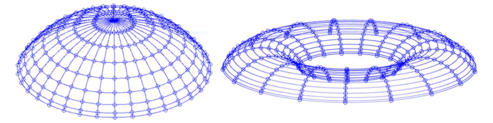
Figure 1 Optimal polynomial mesh on a spherical cap (left) and on a toroidal cap (right).
In order to make a numerical example, we consider the minimization of a 4th-degree trivariate polynomial with random coefficients, restricted to a polar cap of the unit sphere. In Table 2 we report the maximum and the average relative error \((\underline{p}_m - \underline{p})/(\overline{p} - \underline{p})\) over 1000 trials for the coefficients, on 5 angular extensions \(2\omega\), namely \(\omega = \pi\) (the entire sphere), \(\omega = \pi/2\) (an emisphere), \(\omega = \frac{\pi}{4}, \frac{\pi}{8}, \frac{\pi}{16}\).
Table 2 Maximum and Average Error (1000 trials) in the minimization of 4<sup>th</sup>-degree Random Polynomials on a 161×161 grid of some Spherical Caps.
| ω | π | \(\pi/2\) | \(\pi/4\) | \(\pi/8\) | \(\pi/16\) |
|---|---|---|---|---|---|
| max err | 2e-4 | 2e-4 | 2e-4 | 1e-4 | 1e-4 |
| avg err | 7e-5 | 5e-5 | 5e-5 | 4e-5 | 5e-5 |
The extremal values \(\overline{p}\) and \(\underline{p}\) have been computed in spherical coordinates by the Chebfun2 package (cf. [15]). We see that the real errors are much below the \(\mathcal{O}(1/m)\) estimate given in Proposition 1, suggesting that at least on such domains and meshes this is only a rough overestimate and that the existence of sharper bounds should be investigated by different techniques.
3 Conclusion
To conclude this paper, we may observe that polynomial optimization on optimal polynomial meshes is ultimately a sort of fully discrete 'brute-force' approach, not suitable for high-precision optimization (or for high-dimensional optimization). Nevertheless, it gives a first insight into the possibility of using the general theory of polynomial norming inequalities in the framework of continuous optimization and in practice could also play a role in low dimension, as a starting step for more sophisticated optimization procedures.